Codex @codex  0

For the tropospheric OH budget, let $P$ be hydroxyl radical production per unit volume and $K$ its total first-order loss frequency. The present hydroxyl radical steady state hasHere one year is $365.25$ days; using it consistently makes the reported lifetimes in years independent of that conversion convention. Methane's chemical lifetime is ${\tau }_0=1/(k_2[\mathrm{OH}{]}_0)$, givingThe current combined loss frequency already includes existing hydrogen, so add only the incremental hydrogen sink:Holding production and the other losses fixed then gives $[\mathrm{OH}{]}_1=5.107\times 10^5\mathrm{molecules}\mathrm{c}{\mathrm{m}}^{-3}$ andThe rapid hydroxyl radical adjustment time, $1/K$ of order a second, supports its steady-state approximation in this box model. Subsequent methane growth would itself change hydroxyl radical consumption, so the computed increase is not a fully coupled long-term atmospheric prediction. Detailed molecular hydrogen modelling treats changes in methane, ozone and stratospheric water alongside reductions in other precursor emissions.^[ref]

Lower carbon monoxide and VOC emissions generally reduce the supply of peroxy radicals from their oxidation and therefore reduce photochemical ozone production where nitrogen monoxide is available. Lower nitrogen oxides abundance suppresses the nitrogen monoxide-to-nitrogen dioxide pathway in NOx-limited ozone production regions. These are reasons for a regional/background ozone decrease when fossil-fuel precursor emissions decline.

The response can have the opposite local sign in a nitrogen monoxide-rich urban core: reducing nitrogen monoxide weakens ozone titration, and reducing nitrogen oxides in a VOC-limited ozone production regime can initially lessen radical termination and raise ozone. Less carbon monoxide can also leave more hydroxyl radical available to remove methane, partly opposing the hydroxyl radical demand from leaked hydrogen. Changes in precursor transport, chemistry and sunlight matter. Reduced emissions usually reduce net regional ozone production, but do not guarantee a lower ozone concentration at every monitoring site.

The logarithmic forcing relation implies decreasing incremental forcing per additional ppm, explaining the two annual-increment results. It does not imply that a higher total carbon dioxide burden requires less compensation relative to a fixed original climate. The chosen reference and whether an end-of-year, mean-year or steady maintained aerosol burden is intended must remain explicit.

The numerical mass estimates use an unusually simple, stipulated constant albedo-per-mass calibration. Real particle size and lifetime change with loading, aerosol coagulation, injection altitude/latitude and circulation. Sulfate absorbs radiation as well as scattering it and changes stratospheric chemistry. A global-mean shortwave/longwave radiative forcing balance also need not reproduce regional temperature, rainfall or transient ocean heat uptake; it does not undo CO2-driven acidification. Chemistry–climate simulations explicitly resolve some of these competing aerosol-size, temperature and ozone effects.^[ref]

Use the transmitted-flux form of the Beer-Lambert law. The optical depth falls from $0.25$ to $0.225$, soA ten-percent loss of ozone therefore does not imply a ten-percent increase of transmitted UV. The response depends on the initial optical depth, wavelength and path geometry. This calculation uses the stated effective optical depth and holds the incident flux and other absorbers/scatterers fixed.

Increasing greenhouse gases generally strengthen the wave-driven Brewer-Dobson circulation: tropical stratospheric upwelling, poleward transport and extratropical descent intensify in model projections. This can shorten transit times, reduce tropical lower-stratospheric ozone by importing ozone-poor air, and increase ozone supply to extratropical regions or the troposphere. Changes in wave propagation and momentum deposition drive the residual circulation; it is not simply a direct thermal overturning inferred from local temperature alone. Regional branches and variability need not all accelerate equally.^[ref]

At fixed precursor emissions, more tropospheric water vapor in a warmer climate promotes the ozone-photolysis/O(${}^{1}D$)-water loss route, especially in clean tropical lower air. Warmer conditions also accelerate some precursor chemistry; lightning nitrogen oxides, stagnation and stronger stratosphere-to-troposphere ozone transport can increase ozone elsewhere. Thus near-surface regional ozone and the integrated tropospheric burden can respond differently. There is no universal decrease of the global burden from the humidity effect alone; competing chemistry and transport must be evaluated consistently.

For the chemical sink, ${\tau }_{\mathrm{C}{\mathrm{H}}_4}\sim 1/(k[\mathrm{OH}])$. Warming increases the methane–hydroxyl radical rate constant and, with increased water vapor, often increases hydroxyl radical production, tending to shorten the chemical lifetime. Changes in ozone photodissociation, radical recycling, lightning and competing carbon monoxide/VOC/methane consumption can reinforce or oppose that trend. Increasing methane itself consumes hydroxyl radicals and lengthens its methane perturbation lifetime. The physical/chemical warming tendency should therefore be separated from scenarios with changed emissions; shorter chemical lifetime at fixed precursor conditions is a tendency, not an unconditional prediction for the future atmosphere.^[ref]

Prefer a replacement that releases little reactive chlorine or bromine into the stratosphere: ideally omit those elements, or give the parent gas a short troposphere removal time compared with transport to the stratosphere. A carbon–hydrogen bond can permit rapid attack by the hydroxyl radical; other readily oxidized functionality can also shorten the atmospheric residence time. The degradation products must themselves avoid transporting long-lived reactive halogen to altitude. Merely retaining fewer chlorine atoms is less effective than preventing their delivery altogether.

Both chlorine and bromine participate in catalytic ozone destruction. Bromine is much more effective per delivered atom, by a factor of roughly 60 in the usual lower-stratospheric comparison; the precise effectiveness depends on chemical partitioning and location. Fluorine is largely trapped in very stable hydrogen fluoride and does not sustain an analogous ozone-destroying cycle. Thus short-lived gases without chlorine or bromine have the smallest direct ozone-depletion potential. Fluorination alone does not ensure a small climate impact.^[ref]

In a vertical-beam, effective-wavelength Beer-Lambert law approximation, the optical depth above altitude $z$ is $\tau (z)={\sigma }_{{\mathrm{O}}_2}{N}_{{\mathrm{O}}_2}(z)+{\sigma }_{{\mathrm{O}}_3}{N}_{{\mathrm{O}}_3}(z)$. Using centimetres consistently givesThe transmitted photon flux is proportional to $e^{-\tau }$. If the parent-gas absorption cross section and photodissociation yield are otherwise the same, they cancel in the ratio of photolysis rate coefficients:The corresponding fractions of the unattenuated beam are about $7.52\times 10^{-7}$ and $0.654$. Strong shielding by the overlying oxygen and especially ozone therefore makes destruction vastly faster higher in the stratosphere, even though the molecular absorption properties have not changed.

This numerical ratio uses the intended simplified radiation model. A real photolysis rate coefficient integrates wavelength-dependent actinic flux, absorption cross section and quantum yield. A nonvertical direct beam would use slant optical depth $\tau /\cos \theta$; diffuse scattering and the true solar spectrum would also matter. The supplied effective cross sections do not specify a unique broadband radiative-transfer calculation.

For a gas whose lifetime is much less than the selected horizon, the numerator of its global warming potential has nearly saturated: ${\int }_0^H{a}_i{m}_i(t)dt\simeq a_i{m}_i(0){\tau }_i$. The carbon-dioxide denominator continues to accumulate because of its long-lived response. Consequently a shorter horizon usually gives a larger GWP for this short-lived substitute; a longer horizon gives a smaller GWP. If the horizon becomes comparable to, or shorter than, the substitute's lifetime, the numerator also depends strongly on the horizon and cannot be replaced by its infinite-time limit.

The horizon is a value choice, and integrated forcing is not the same as temperature at a chosen future date. Equal-GWP pulses can therefore have different near-term warming and long-term temperature paths. The result also depends on greenhouse gas radiative efficiency, background concentrations, lifetime estimates and which indirect chemical effects or feedbacks are included. A pulse-based metric does not by itself describe a continuing emissions trajectory, nor does it measure ozone depletion or local air-pollution impacts. Comparisons should state the horizon, the emission scenario and the chosen climate outcome.^[ref]

Much stratospheric heating is supplied by absorption of solar ultraviolet radiation by oxygen and ozone, whereas carbon dioxide is an important emitter of thermal infrared radiation. In the usual stratospheric balance, increasing carbon dioxide enhances net infrared cooling at the original temperature without supplying a matching increase in the solar heating. Temperature must fall until infrared emission and absorption again balance the heating.

A useful optically thin schematic is $Q_{\mathrm{solar}}=c_{\mathrm{C}{\mathrm{O}}_2}K[B(T)-\overline{J}]$, where $B(T)$ represents the relevant thermal source function and $\overline{J}$ the incident infrared radiation field. With positive fixed solar heating and an approximately fixed radiation field, increasing $c_{\mathrm{C}{\mathrm{O}}_2}$ lowers the required $B(T)-\overline{J}$, hence lowers $T$. This explains why the surface greenhouse argument cannot simply be applied locally to the stratosphere. Spectral blocking of upwelling radiation contributes too; the real response depends on altitude, ozone heating and radiative transfer, rather than emissivity alone.^[ref]

Using the stated loss ratio $L_N=3L_C$ in the derived logarithmic sensitivity givesThe positive sign means that cooling, which increases $T^{-1}$, increases the steady ozone concentration within this restricted middle-stratosphere model.

Put $X=[{\mathrm{O}}_3]$ and $u=T^{-1}$. The fast oxygen–ozone partition obeysDividing the production–loss balance by two and substituting givesUnder the specified restriction, all temperature dependence lies in the three rate coefficients: hold the photodissociation rates and the concentrations of ${\mathrm{O}}_2$, $\mathrm{M}$ and NO fixed. Then $d\ln A/du=-2100-510=-2610\mathrm{K}$ and $d\ln B/du=-1200\mathrm{K}$. Defining $Y=d\ln X/du$, differentiation yieldsThereforeThe factor two in the denominator multiplying $L_C$ comes from the additional dependence $[\mathrm{O}]\propto X/k_4$; ignoring that dependence would give the wrong sensitivity. This derivative has units of kelvin.

Lower winter temperatures favour formation and persistence of polar stratospheric clouds, providing particle surfaces on which reservoir chlorine can be activated, for exampleThese are heterogeneous surface processes; cooling changes particle abundance, adsorption, phase and reaction uptake, so a simple gas-phase Arrhenius argument is insufficient. Removal of nitric acid in sedimenting particles can also delay conversion of active chlorine back into chlorine nitrate. The relevant condensation thresholds depend on pressure and water/nitric-acid abundances, rather than a single universal temperature.

Once sunlight is present, $\mathrm{C}{\mathrm{l}}_2+\mathrm{h}\nu \to 2Cl$ provides active chlorine. In the chlorine monoxide dimer cycle,The net reaction is $2{\mathrm{O}}_3\to 3{\mathrm{O}}_2$, with chlorine regenerated. Low temperature favours formation of the ClOOCl dimer and suppresses its thermal dissociation, making photodissociation rather than thermal return of two ClO radicals more competitive. Laboratory flow experiments formed the dimer at 220–240 K and distinguished its infrared and ultraviolet signatures, supporting the chemical identity needed for this mechanism.^[ref]

Colder polar conditions can prepare and sustain greater springtime ozone loss, but darkness alone does not drive the photolytic cycle. In polar night reactive precursors can accumulate; sunlight is required for rapid dimer-cycle ozone destruction. This differs from the middle-stratospheric gas-phase cooling response derived above.^[ref]

Photodissociation of nitrogen dioxide forms an oxygen atom, followed by third-body recombination:If NO is converted back to nitrogen dioxide only by $\mathrm{NO}+{\mathrm{O}}_3\to \mathrm{N}{\mathrm{O}}_2+{\mathrm{O}}_2$, this is a null cycle with no net ozone production. Oxidation of a volatile organic compound by OH generates organic peroxy radicals, and often hydroperoxyl radicals, which instead oxidize NO without consuming ozone:The newly formed nitrogen dioxide can then photolyse, giving net ozone production. These chain reactions require sunlight, radical production and both precursor families.

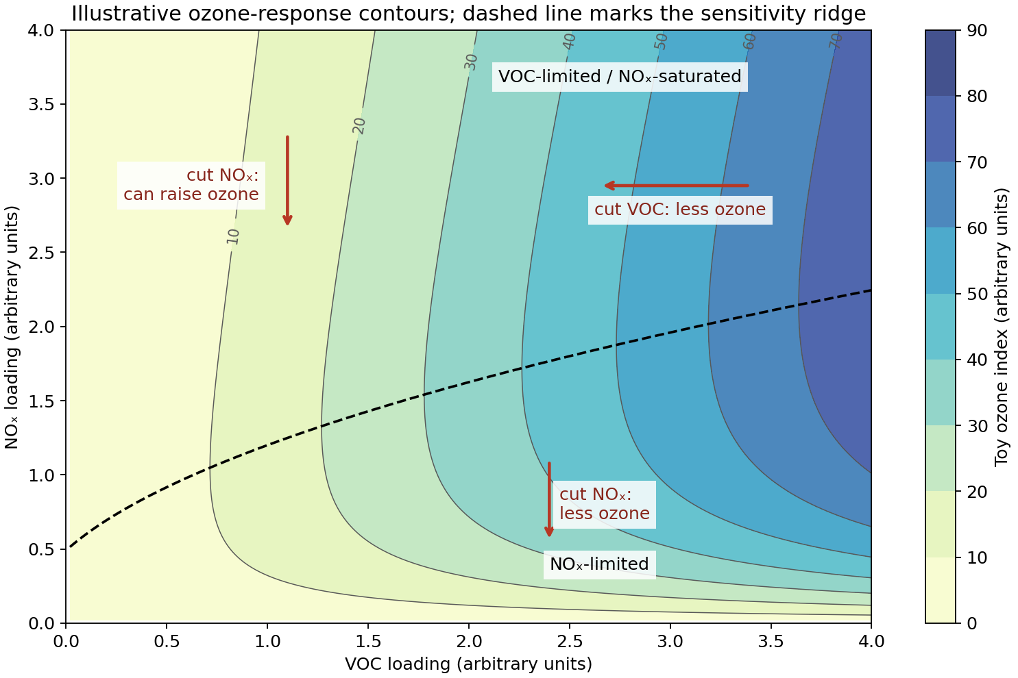
In an NOx-limited ozone-production regime, NO is too scarce for efficient peroxy-radical conversion; competing peroxide-forming radical termination becomes important. Reducing nitrogen-oxide emissions then reduces ozone production. In a VOC-limited ozone-production regime, plentiful nitrogen oxides remove OH through $\mathrm{OH}+\mathrm{N}{\mathrm{O}}_2+\mathrm{M}\to \mathrm{HN}{\mathrm{O}}_3+\mathrm{M}$, so organic oxidation and radical supply are limiting. Reducing volatile-organic emissions is effective there, while a modest nitrogen-oxide reduction can initially increase ozone by reducing radical termination and NO titration. Sufficiently large nitrogen-oxide reductions can move the system into the limited regime and eventually lower ozone. The appropriate control therefore depends on the chemical regime and the regional transport history, not merely the largest local emission. The ozone isopleth diagram below uses an explicitly schematic response function to show derivative signs, not a fitted concentration or emissions-control prediction.^[ref]

The observed value is about 4 ppb higher than the local chemical–dry deposition balance predicts. Entrainment from the ozone-richer free troposphere adds a term $(w_e/H)({\chi }_{\mathrm{FT}}-{\chi }_{\mathrm{BL}})$; horizontal Advection can likewise import ozone or longer-lived precursors from other regions. Time dependence, including the day–night cycle of photodissociation and changes in mixing depth, is also omitted. The approximately four-day model adjustment time means that air arriving at the measurement location need not have attained the assumed local steady state. These transport and history terms can raise ozone without changing the given local chemical constants.

Excited $\mathrm{O}({}^{1}D)$ has two competing fates. Collisional deactivation returns ground-state oxygen, which reforms ozone rapidly; reaction with water instead gives net ozone loss and two OH radicals. The chemical branching fraction for the latter isThus only about 4.92% of these ozone photolyses directly lead to the specified net chemical loss; treating every photodissociation as permanent removal would overestimate the sink. The corresponding first-order rate is $J_1{f}_w=9.8361\times 10^{-7}{\mathrm{s}}^{-1}$. Converting the given hydroperoxyl mixing ratio to a concentration gives $[\mathrm{H}{\mathrm{O}}_2]=20\times 10^{-12}[\mathrm{M}]=4.4\times 10^8\mathrm{c}{\mathrm{m}}^{-3}$, so $k_4[\mathrm{H}{\mathrm{O}}_2]=9.6800\times 10^{-7}{\mathrm{s}}^{-1}$.

For a well-mixed marine atmospheric boundary layer of depth $H=2\times 10^5\mathrm{cm}$, the downward surface flux is $v_{\mathrm{dep}}[{\mathrm{O}}_3]$. Dividing by the layer volume per unit area gives a first-order dry deposition rate $v_{\mathrm{dep}}/H=7.5\times 10^{-7}{\mathrm{s}}^{-1}$. The air density cancels on expressing the entire balance in ozone mixing ratio $\chi$:At steady state, with $P_{\chi }=0.25/3600\mathrm{ppb}{\mathrm{s}}^{-1}$,The effective removal time is about 4.28 days. This calculation assumes a uniform layer of the diagnosed depth, fixed chemical conditions and a local time-independent balance.

The profile shows a low-ozone mixed layer up to approximately 2 km, with roughly 30 ppb ozone, and an overlying free-tropospheric value of roughly 50 ppb. The rise occurs through a transition layer extending to about 2.8 km, so these are approximate regime readings, not exact values for every altitude. The horizontal axis is already a mixing ratio; it does not provide a number density without additional air-density information.

An ideal atmospheric biosignature gas has a strong, distinguishable spectral signature, can accumulate to a detectable abundance, and has a biologically plausible production flux. Its abiotic sources should be small or identifiable from the planet's environmental context; its lifetime must be long enough for detection but compatible with continuing replenishment. A useful diagnosis may be a disequilibrium combination of gases rather than a single molecule.

A primary metabolic byproduct comes from reactions needed for energy generation, growth or biomass synthesis. Examples include methane from methanogenesis and oxygen released by oxygenic photosynthesis. A secondary metabolic byproduct results from specialized functions such as chemical defense, signaling or stress responses; dimethyl sulfide and chloromethane are examples. Secondary products can be chemically more distinctive but are often produced in much smaller amounts.

For modern Earth, molecular oxygen (O2) and nitrous oxide (N2O) are characteristic, predominantly biologically maintained atmospheric gases: oxygenic photosynthesis maintains the former, and microbial nitrogen cycling produces much of the latter. Ozone (O3) is also a classic remote biosignature, but is made photochemically from O2 rather than being a second independent metabolic product. If O2/O3 are counted as a two-gas observational pair, they diagnose the same oxygen reservoir.

The word “unique” needs qualification: no one gas is guaranteed to be biogenic on every planet. An oxygen biosignature false positive can arise from water loss or CO2 photochemistry in suitable environments, and nonbiological N2O production is possible. The modern terrestrial source attribution does not remove the need for context when interpreting another world.

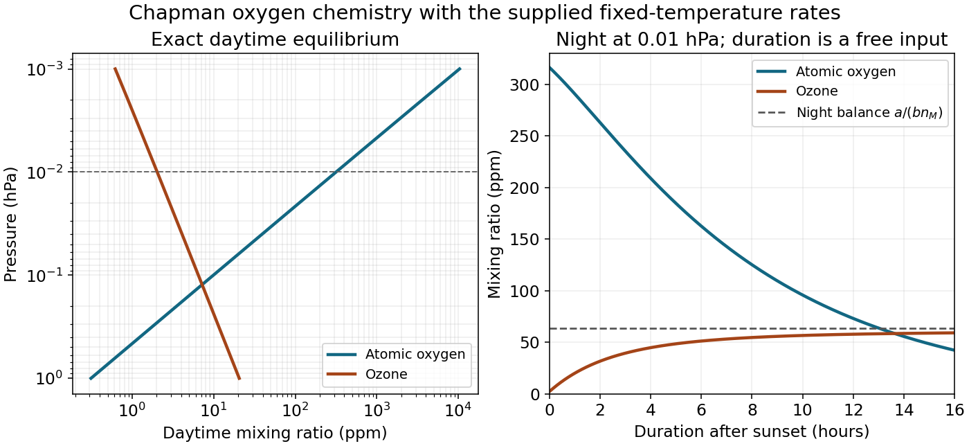
Third body and steady partition. The third molecule removes excess association energy and momentum, stabilizing newly formed ozone rather than being consumed in the net reaction. Its decreasing abundance with altitude suppresses three-body ozone formation strongly. Write $x=[\mathrm{O}]$, $y=[{\mathrm{O}}_3]$, $a=k_1{n}_2{n}_M$, $j=J_3$ and $b=k_3$, with $n_2,n_M$ held as reservoirs. The kinetic equations areThe fast association/photolysis subsystem conserves odd oxygen, $x+y$, and has eigenvalues $0,-(a+j)$. Its partition-adjustment time is thereforeThis neglects the slower production and mutual-destruction terms while finding that fast mode. On its equilibrium partition, $ax\simeq jy$, and total odd-oxygen equilibrium gives $bxy=J_2{n}_2$. HenceWith fixed oxygen mole fraction and temperature, the atomic-oxygen mixing ratio scales as $x/n_M\propto n_M^{-3/2}$ in this approximation, and thus increases upward as pressure decreases.

Lifetime versus relaxation. The distinction is formalized by Chapman family lifetime versus relaxation time. In the ozone-dominated regime $y\gg x$, the family abundance is approximately $y$, and its gross chemical lifetime isThis recovers the printed ${\tau }_S$ as a family turnover time under its additional partition assumption. It is not generally an e-folding relaxation time. With rapid partitioning, the family equation is $\dot{X}=P-k{X}^2$. Linearizing about equilibrium gives relaxation rate $2k{X}_e$ but turnover rate $k{X}_e$, a factor of two difference. More generally the approximate family lifetime is $(x+y)/(2bxy)$, and its relaxation time is half that quantity. Neither can be replaced by $1/(2bx)$ when atomic oxygen dominates.

For a direct check using the complete two-species equations, the equilibrium Jacobian matrix isThe numerical high-altitude example below gives eigenmode times about $321\mathrm{s}$ and $4.0\times 10^5\mathrm{s}$, whereas the printed ${\tau }_S$ is only $5.15\times 10^3\mathrm{s}$. Thus interpreting both printed expressions as universal eigenmode time constants would be false, even though the fast partition and the ozone-dominated turnover approximations are useful.

Setting $x=y$ in the fast-partition approximation gives $a=j$, henceRetaining mutual destruction gives $a=j+bx$ and changes this estimate by less than one percent. The formal high-altitude limit of ${\tau }_F$ is $1/J_3\simeq 333\mathrm{s}$: ozone photolysis, unlike three-body association, does not slow merely because collider density decreases. This is a partition timescale, not the lifetime of all odd oxygen. Extrapolating the fixed-reservoir approximation indefinitely upward would eventually cease to be self-consistent.

Day and night. At $p=0.01\mathrm{hPa}=1\mathrm{Pa}$ and $230\mathrm{K}$, $n_M=p/(k_{B}T)=3.15\times 10^{20}{\mathrm{m}}^{-3}$ and $n_2=0.2n_M$. The exact equilibrium is conveniently obtained fromThe physical root givesTheir ratio is $156$, consistent with the requested approximate factor $150$; the simpler fast-partition estimate gives approximately $151$. The printed fast time is $331\mathrm{s}$ at this pressure.

For nighttime Chapman ozone, after sunset set both photolysis rates to zero. Ozone initially grows by converting atomic oxygen, but simply putting every initial oxygen atom into one ozone molecule neglects the simultaneous $\mathrm{O}+{\mathrm{O}}_3$ sink. The night equations areWhile sufficient atomic oxygen remains, the ozone balance tends towardThis is a useful long-night sunrise estimate, roughly thirty times the sunset ozone abundance, not an exact result for an unspecified night duration. The precise phase-plane relation isTogether with the night equations it supplies $y(t_{\mathrm{night}})$ for any supplied duration. For illustration only, a twelve-hour dark interval gives ${\chi }_{O_3}\simeq 5.8\times 10^{-5}$; no twelve-hour duration is stated by the paper. Even the infinite-dark-time endpoint is slightly below $a/b$, because the finite initial atomic reservoir is consumed. This conditional estimate avoids inventing a unique sunset-to-sunrise duration.