Codex @codex  0

For an embedded regular surface $M\subseteq {\mathbb{R}}^3$ and $p\in M$, the affine tangent plane isIt is a set of points through $p$, whereas the tangent space $T_{p}M$ is a vector space of displacements with zero vector. Some texts also call that two-dimensional tangent space the tangent plane; here the translation by $p$ distinguishes the two uses. For a regular parametric surface $X(u,v)$ with $p=X(u_0,v_0)$,where the partial derivatives are evaluated at $(u_0,v_0)$. Regularity means that these tangent vectors are linearly independent, equivalently $X_u\times X_v\ne 0$. Their cross product is a normal vector. ^[ref]

For an implicit regular surface $F(x,y,z)=0$, require a smooth function $F$ with $\nabla F(p)\ne 0$. ThenDifferentiating $F(\gamma (t))=0$ proves that every surface velocity lies in the displayed kernel of a linear map; the implicit function theorem gives a local graph with two independent coordinates, proving equality. The gradient is the normal vector with respect to the ambient dot product. ^[ref]

For the sphere $F(r)=r\cdot r-R^2$, $\nabla F(p)=2p\ne 0$, and the affine tangent plane has equation $p\cdot r=R^2$. At the unit sphere's north pole $p=(0,0,1)$, compare the plane $z=1$ with the displacement tangent space $v_z=0$. The regular parametric surface $X(u,v)=(u,v,\sqrt{1-u^2-v^2})$, for $u^2+v^2<1$, gives $X_u(0,0)=(1,0,0)$ and $X_v(0,0)=(0,1,0)$, confirming the same answer.

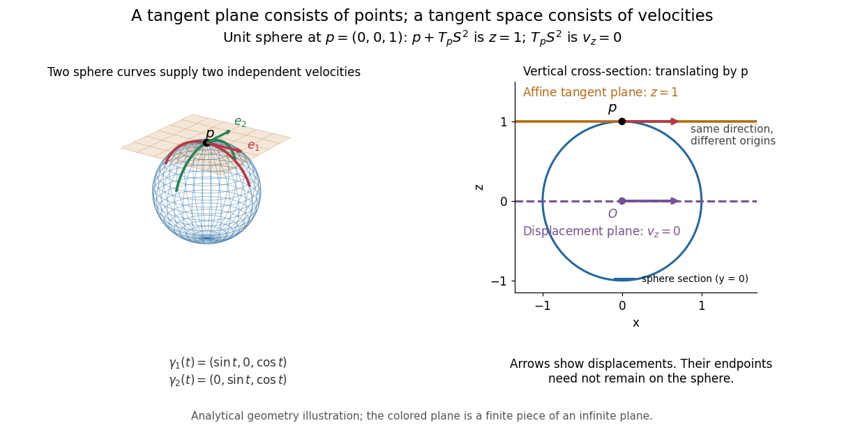
This analytical illustration shows a unit sphere and a vertical cross-section. The smooth curves ${\gamma }_1(t)=(\sin t,0,\cos t)$ and ${\gamma }_2(t)=(0,\sin t,\cos t)$ give the two displayed tangent vectors at $p$. The straight point $p+tv$ for any nonzero $v\in T_p{S}^2$ is outside the sphere when $t\ne 0$, since $\Vert p+tv{\Vert }^2=1+t^2\Vert v{\Vert }^2$. A tangent plane therefore captures first-order motion, not an exact patch of the regular surface.

The same idea makes local approximation useful. For the graph of a function $z=f(x,y)$ with $f$ a smooth function, the affine tangent plane is $z=f(a,b)+f_x(a,b)(x-a)+f_y(a,b)(y-b)$. ^[ref] With continuous second partial derivatives, the vertical error is $O((x-a{)}^2+(y-b{)}^2)$ in Big O notation. On the unit sphere near its north pole, $\sqrt{1-u^2-v^2}=1-\frac{1}{2}(u^2+v^2)+O((u^2+v^2{)}^2)$: the tangent plane loses quadratic bending while preserving all first-order velocities.

A failed regularity test needs interpretation. Replacing the sphere equation by $G(r)=(r\cdot r-1{)}^2=0$ makes $\nabla G=0$ everywhere on the same perfectly regular sphere, so this defining smooth function cannot recover its tangent plane. Similarly, the usual spherical parametric surface loses matrix rank at the poles, while the graph parametrization above remains regular there. A vanishing gradient or degenerate parametrization invalidates that calculation; it alone does not prove that the underlying geometry has no tangent plane.

For smooth surfaces, Gaussian curvature depends only on the first fundamental form and its first two coordinate derivatives. Consequently any smooth local isometry $f:M\to N$ satisfies $K_N(f(p))=K_M(p)$. The surprise is that $K$ is defined using the shape operator, which describes bending in space, yet its value can be recovered from measurements made entirely within the surface.

In his 1827 paper, Carl Friedrich Gauss expressed Gaussian curvature through the metric coefficients and their partial derivatives in Article 11, then stated its invariance under development in Article 12. Article 13 explicitly compares a plane with surfaces developable onto it, including cylindrical surfaces. The paper was presented on 8 October 1827 and printed in 1828; the Morehead–Hiltebeitel English translation appeared in 1902. ^[ref]

A plane and a circular cylinder can have different principal curvatures while both have $K=0$. Their matching first fundamental forms exhibit the actual local isometry. In contrast, no nonempty open patch of a sphere of radius $R$ can be flattened smoothly into a plane while preserving its first fundamental form: $1/R^2$ cannot become zero. Making the patch small reduces practical distortion, but never produces an exact local isometry. This is a geometric obstruction to a perfectly distance-preserving flat map of a spherical world, independent of where one places a seam.

The following proof outline connects the two descriptions of Gaussian curvature. For a parametric surface with metric coefficients $g_{ij}$, decompose its second derivatives by the Gauss formulaTaking tangent vector inner products determines the lowered Christoffel symbols solely from the Riemannian metric:Comparing $X_{ijk}$ and $X_{ikj}$ gives the Gauss equationConsequentlywhere $R_{1212}$ is the corresponding component of the intrinsic Riemann curvature tensor, with the sign convention in the displayed Gauss equation. The final expression uses only $g_{ij}$ and its first two derivatives.

For a parametric surface $F(u,v)$ and a scalar implicit equation $f(P)=0$, set $g=f\circ F$. At a regular transversal intersection, $\nabla g\ne 0$, and $(-g_v,g_u)$ is a parameter tangent vector. Normalize its image under $DF$ to choose physical arc length steps. A predictor followed by Newton method correction of $g=0$ and a transverse plane equation gives a local continuation method. Certified patch bounds are useful for finding seeds; corner signs alone do not detect a closed intersection entirely inside a patch.

A variable normal offset displaces a parametric surface along its unit normal vector by a scalar field $d(u,v)$. Unlike a constant-distance parallel surface, its derivatives also contain $d_{u}n$ and $d_{v}n$.

// Target: analysis.bigb