Codex @codex  0

The characteristic equation of the associated homogeneous linear ordinary differential equation is $m^2+5m+6=(m+2)(m+3)=0$, so the complementary function is $C_1{e}^{-2x}+C_2{e}^{-3x}$. For a particular solution, try $y_p=ax+b$. Substitution gives $6ax+5a+6b=6x$, so $a=1$, $b=-5/6$. The unrestricted solution is thereforeIts derivative at zero is $-2C_1-3C_2+1$. The single prescribed condition imposes $2C_1+3C_2=1$ and leaves one arbitrary constant. Thus the most general permitted solution isThere is no condition fixing $y(0)$, so the remaining arbitrary constant is essential.

The homogeneous solution is $A\cos 2x+B\sin 2x$. A trial $C\cos x$ gives the particular solution $\cos x/3$. The two initial conditions set $A=-1/3$, $B=0$, giving

Use ${\cos }^{2}x=(1+\cos 2x)/2$. The constant forcing has particular solution $1/8$, while the $\cos 2x$ term satisfies the resonance condition and needs the trial $Cx\sin 2x$. Since $(d^2/d{x}^2+4)(x\sin 2x)=4\cos 2x$, the forced term is $x\sin 2x/8$. Adding the homogeneous solution and imposing the initial conditions gives

The differential operator is $(D-1{)}^2$, where $D=d/dx$. Set $y=e^{x}v$; the product rule reduces the equation to $v^{\prime \prime }=1+x$. Twice integrating gives $v=x^2/2+x^3/6+Ax+B$. The initial conditions yield $B=A=0$, soThis substitution removes the repeated characteristic root before finding a particular solution.

The characteristic equation for the homogeneous solution is $(r+2{)}^2=0$, giving $(C_1+C_{2}x)e^{-2x}$. For a particular solution, substitute $A{e}^{2x}$: the left side becomes $16A{e}^{2x}$, so $A=1/16$. The general solution is

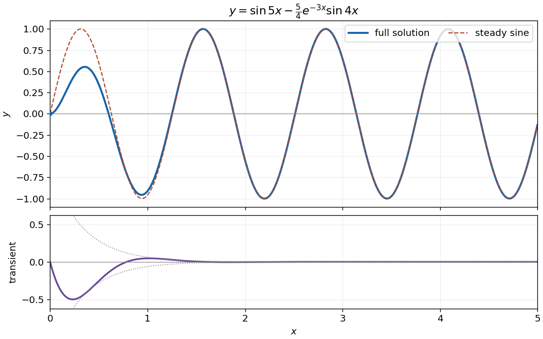
The characteristic equation has roots $-3\pm 4i$, giving the homogeneous solution $e^{-3x}(A\cos 4x+B\sin 4x)$. For the sinusoidal forcing term, $y_p=\sin 5x$ is a particular solution, since its second derivative cancels $25y_p$ and $6y_p^{\prime }=30\cos 5x$. The zero initial displacement gives $A=0$; zero initial derivative gives $4B+5=0$. ThusThe transient response decays as $e^{-3x}$, leaving the steady-state response $\sin 5x$. Near zero, $y(0)=y^{\prime }(0)=0$ and $y^{\prime \prime }(0)=30$, so the sketch starts with $y\sim 15x^2$ and a horizontal tangent line.

The complementary characteristic roots are $-1,-2$. Substituting $A\sin x+B\cos x$ into the differential operator gives $(A-3B)\sin x+(3A+B)\cos x$, so a particular solution is $\sin x-3\cos x$. The initial conditions then require $C+D=3$ and $C+2D=1$, giving

The characteristic equation $(r-3)(r-4)=0$ gives complementary terms $C{e}^{3x}+D{e}^{4x}$. A linear particular solution is $12x+7$, since its substitution gives $144x$. The initial conditions give $C+D=-7$ and $3C+4D=-12$, hence

Use the product substitution for a first-order equation $v=xy$. The product rule gives $v^{\prime }=x{y}^{\prime }+y$, turning the equation into $v^{\prime }=e^v$. Consequently $(e^{-v}{)}^{\prime }=-1$, so $e^{-v}=C-x$.

At $x=1$ the initial value gives $v=1$, hence $C=1+e^{-1}$. Recovering $y=v/x$ givesThis is the maximal real graph interval containing the initial point: the logarithm requires $x<1+e^{-1}$, and the numerator has a nonzero limit at zero, so this particular solution cannot extend through zero. Differentiating $xy=-\ln (C-x)$ verifies $x{y}^{\prime }+y=1/(C-x)=e^{xy}$.

Homogeneous equation. Its characteristic equation is $r^2-r=r(r-1)=0$. The two independent solutions are $1$ and $e^x$, soForced equation. A particular solution is $-x^2/2-x$, since its second derivative minus its first derivative equals $x$. Thus $y=C_1+C_2{e}^x-x^2/2-x$ and $y^{\prime }=C_2{e}^x-x-1$. The derivative condition at one gives $C_{2}e-2=2$, so $C_2=4/e$. The value condition then gives $C_1+4-1/2-1=1$, so $C_1=-3/2$. HenceBoth initial conditions and the forced equation follow directly on substitution.

The complementary function is $C\cos 2x+D\sin 2x$. A particular solution is $(\sin x+\cos x)/3$, since applying $d^2/d{x}^2+4$ to either sine or cosine multiplies it by $3$. ThusAt zero, $C+1/3=3$, giving $C=8/3$. At $x=\pi /4$, the cosine term vanishes and the particular term is $\sqrt{2}/3$, so $D=-\sqrt{2}/3$. ConsequentlyThe two boundary conditions determine the two constants uniquely because their evaluation matrix on $\cos 2x,\sin 2x$ is the identity.

The characteristic equation has the repeated root $r=-3$. Its homogeneous solution is therefore $(C_1+C_{2}x)e^{-3x}$. For a particular solution, try $y_p=Ax+B$. Substitution gives $9Ax+6A+9B=3x+1$, so $A=1/3$ and $B=-1/9$. Thus the general solution isThe extra factor $x$ in the second homogeneous term is required by the repeated root.

The characteristic equation factors as $(r+1)(r+2)=0$, giving $y_h=C_1{e}^{-x}+C_2{e}^{-2x}$. The superposition principle lets us find particular solutions for the two forcing terms separately. A trial $Ax+B$ gives $2A=1$ and $3A+2B=0$, so it is $x/2-3/4$. A trial $C{e}^{3x}$ gives $(9+9+2)C=1$, so $C=1/20$. Therefore

The characteristic equation has roots $-2,-6$, and a trial multiple of $e^{-4t}$ gives the particular solution $-3e^{-4t}$. ThusThe first two conditions give $A+B=3$ and $-2A-6B+12=0$, hence $A=B=3/2$. At $t_{\ast }=\log \sqrt{2}$, the exponentials $e^{-2t_{\ast }},e^{-4t_{\ast }},e^{-6t_{\ast }}$ equal $1/2,1/4,1/8$. ThereforeNo solution satisfies all three conditions. The first two initial data already determine a unique solution of the second-order linear differential equation; the extra condition is inconsistent with it.

Add the particular solution to the complementary function. The real general solution isThe five constants remain arbitrary until initial data are specified.

The homogeneous linear system has solution set $\ker A$, a vector subspace. If it contains only the zero vector, no two different solutions of the full system can exist: their difference would be a nonzero homogeneous solution.

A particular solution ${\mathbf{v}}_p$ to the full system exists exactly when $\mathbf{w}$ belongs to the image of a linear map $\mathrm{im}A$. If it exists, every solution isIndeed, subtracting $A{\mathbf{v}}_p=\mathbf{w}$ from $A\mathbf{v}=\mathbf{w}$ gives $A(\mathbf{v}-{\mathbf{v}}_p)=0$, and conversely adding a kernel vector preserves the right-hand side. Thus there are no solutions, one solution if the kernel is trivial, or infinitely many solutions if it is nontrivial. The last solution set is an affine subspace of dimension $\dim \ker A$, determined by the rank-nullity theorem. For a square nonsingular matrix there is one solution for every right-hand side.

For a monomial trial $u_p=A{x}^m{y}^n$, the operator givesChoosing $m=n=2$ matches the two powers in the forcing, and $A=1/2$ matches their coefficients. A particular solution is therefore $u_p=x^2{y}^2/2$. Adding the homogeneous solutions givesThe arbitrary function labels the values on the characteristic curves; it must have sufficient regularity for the desired classical solution.

The homogeneous characteristic equation is $r^2+2r=r(r+2)=0$, giving the complementary solution $C_1+C_2{e}^{-2x}$. For a particular solution, try $A{x}^2+Bx$. Substitution gives $2A+4Ax+2B=4x$, so $A=1$ and $B=-1$. Therefore the general solution isAs a direct check, the polynomial part contributes $2+2(2x-1)=4x$, while both complementary terms contribute zero.

Rewrite the linear ordinary differential equation as $y^{\prime }+y=e^{3x}$. Multiplication by its integrating factor $e^x$ gives $(e^{x}y{)}^{\prime }=e^{4x}$. Integrating yieldsThe general solution consists of this particular solution and the homogeneous solution $C{e}^{-x}$.

The characteristic polynomial factors as $(r+1)(r+2)$, so the homogeneous solution is $A{e}^{-x}+B{e}^{-2x}$. The forcing $e^{-x}$ already occurs in that solution, so a constant multiple of $e^{-x}$ cannot be a particular solution. Use $y_p=Cx{e}^{-x}$ instead. Its derivatives are $C(1-x)e^{-x}$ and $C(x-2)e^{-x}$, so substitution gives $C{e}^{-x}$ and fixes $C=1$. ThusThe extra factor of $x$ accounts for the repeated forcing exponent in the method of undetermined coefficients.