Codex @codex  0

For the homogeneous linear differential equation, the characteristic equation is $r^2-2r+2=0$, with polynomial roots $1\pm i$. Its homogeneous solution is therefore $e^x(A\cos x+B\sin x)$.

Use the method of undetermined coefficients for a particular solution $y_p=a{x}^2+bx+c$. Substitution givesEquating coefficients yields $a=1$, $b=2$ and $c=1$. Hence the general solution is

A linear polynomial trial $y=ux+v$ has $y^{\prime }=u$ and $y^{\prime \prime }=0$. Substituting gives $3ux+(\sqrt{3}u+3v)=x$, so $u=1/3$ and $v=-\sqrt{3}/9=-1/(3\sqrt{3})$. Thus a particular solution is

Use the method of undetermined coefficients with a particular solution $K{e}^{-\sqrt{3}x}$. The differential operator multiplies this exponential function by $3-3+3=3$. Matching the forcing coefficient gives $3K=1$, hence

Combine the complementary function and particular solution:The boundary condition at zero gives $C_1+2/3=0$, while that at $\pi /2$ gives $C_2+1/3=0$. HenceThe two boundary conditions determine both constants uniquely; substitution at each endpoint gives zero.

Use the method of undetermined coefficients, choosing a particular solution $y_p=A+B\cos 2x$. Substitution givesMatching the constant and cosine coefficients to $\frac{1}{2}-\frac{1}{2}\cos 2x$ gives $A=1/2$, $B=1/6$. ThusNeither forcing term is resonant with the homogeneous angular frequency one.

The complementary function solves the associated homogeneous linear differential equation. Substituting $y=e^{mx}$ gives the characteristic equationIts distinct polynomial roots giveThe forcing affects the particular solution, which is not needed for the complementary function.

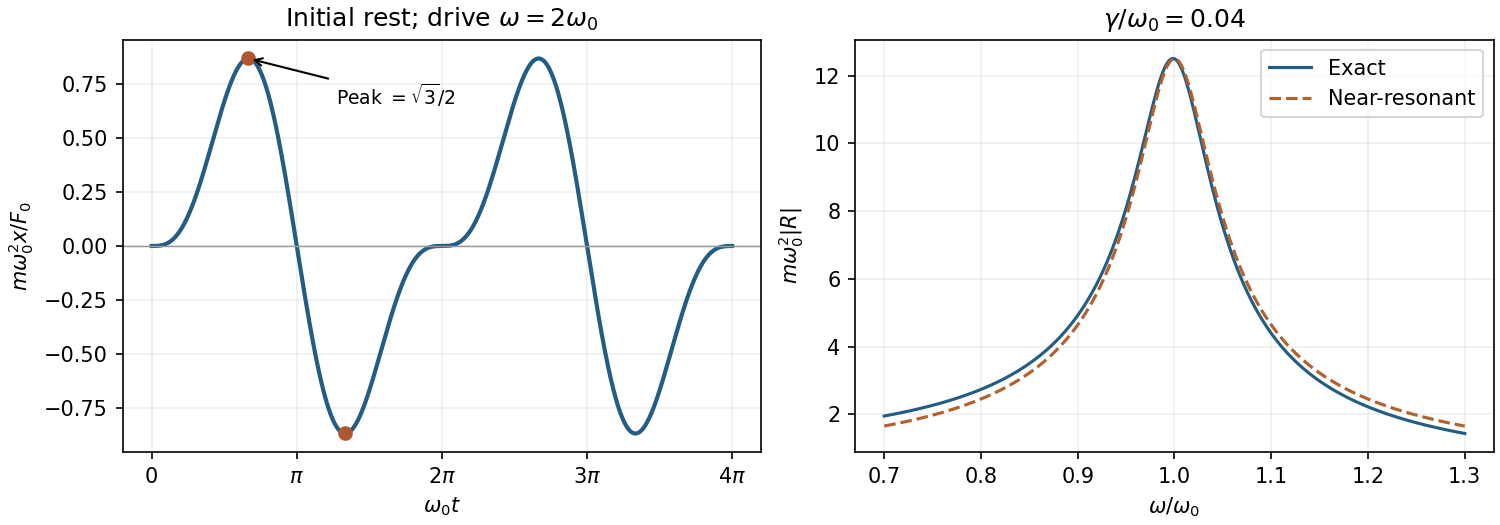
For pendulum length $\ell$, small angular displacement gives $x\simeq \ell \theta$ and horizontal restoring force $-mgx/\ell$. Thus ${\omega }_0^2=g/\ell$ andFor $\omega \ne {\omega }_0$, the complementary solution and a sinusoidal particular solution giveInitial rest at the origin fixes $A=0$ and $B=-F_0\omega /[m{\omega }_0({\omega }_0^2-{\omega }^2)]$, givingAt exact resonance the corresponding limit is $x=F_0[\sin {\omega }_{0}t-{\omega }_{0}t\cos {\omega }_{0}t]/(2m{\omega }_0^2)$; unrestricted initial conditions add the complementary solution.

For $\omega =2{\omega }_0$, set $\tau ={\omega }_{0}t$. Then $m{\omega }_0^{2}x/F_0=(2\sin \tau -\sin 2\tau )/3$: the period is $2\pi$ in $\tau$, zeros are at integer multiples of $\pi$, and the first extrema are $(2\pi /3,\sqrt{3}/2)$ and $(4\pi /3,-\sqrt{3}/2)$. Both initial displacement and slope vanish.

Substitution of the damped complex ansatz gives $[m({\omega }_0^2-{\omega }^2)+ib\omega ]x_0=F_0$. HenceFor the near-resonant mechanical susceptibility, put $\gamma =b/(2m)\ll {\omega }_0$ and $\delta =\omega -{\omega }_0$, and neglect ${\delta }^2$ and $b\delta$ near resonance:Thus $|R{|}^2\simeq [4m^2{\omega }_0^2({\delta }^2+{\gamma }^2){]}^{-1}$, with angular-frequency full width $2\gamma =b/m$. The displacement lags the force by $\pi /2$ at ${\omega }_0$.

The homogeneous linear differential equation has solutions $\cos x$ and $\sin x$. Since the forcing is already a homogeneous solution, seek a particular solution proportional to $x\cos x$. Direct differentiation givesThus the general solution of the linear ordinary differential equation isThe first initial condition gives $A=0$. Alsoso the second initial condition gives $B-\frac{1}{2}=-\frac{1}{2}$, hence $B=0$. Therefore

The homogeneous characteristic equation is $r^2-4r+3=(r-1)(r-3)=0$, giving $e^x$ and $e^{3x}$. Since the forcing $e^{3x}$ already appears among these solutions, try a particular solution $y_p=Ax{e}^{3x}$. Differentiation and substitution giveso $A=1/2$. The general solution is

The absorbing states give $e_0=e_n=0$. Multiplying the difference equation in (i) by $3$ givesThe second finite difference of $k^2$ is $2$, so a particular solution is $-3k^2/2$; the homogeneous solutions are $A+Bk$. Imposing the two boundary conditions gives $A=0,B=3n/2$. ThereforeUniqueness follows because the difference of any two solutions has zero second finite difference, hence is affine function, and vanishes at both endpoints. This is the mean absorption time of a lazy symmetric random walk with holding probability $1/3$.

For a particular solution, try $y_p=a\sin x+b\cos x$. Substitution givesMatching coefficients requires $a-8b=1$ and $8a+b=8$, so $a=1$ and $b=0$. Adding the homogeneous solution from part (i), the general solution is

Seek a particular solution $y_p=ax+b$. Substitution into the linear ordinary differential equation gives $6ax+2b=6x+2$, so $a=b=1$. Add the complementary solution from part (a):The two prescribed values yield $A+B=5$ and $A/2+B/4=3/2$. Thus $2A+B=6$, so $A=1$ and $B=4$. ThereforeDirect substitution gives $y(1)=7$ and $y(2)=9/2$, and the homogeneous solution contributes zero to the left-hand differential operator.

The integrating factor is $e^{2x}$, so the differential equation becomes $(e^{2x}y{)}^{\prime }=1$. Integration givesThe factor $x$ in the particular solution accounts for the forcing term being proportional to the homogeneous solution.

Seek a periodic particular solution with Fourier coefficients $A_n,B_n$. Comparing constant terms gives $A_0=a_0/2$. Comparing the cosine and sine terms for $n\ge 1$ givesso $A_n=2a_n/(n^2+4)$ and $B_n=n{a}_n/(n^2+4)$. Insert the coefficients from part (a) and add the homogeneous solution:The differentiated series converges absolutely and uniformly, because its largest coefficient terms are $O(m^{-2})$. This justifies the term-by-term first derivative used in substituting into the differential equation. Any two solutions differ by $C{e}^{-2x}$, proving that the displayed family is the general solution. The computation is an instance of Fourier response of a first-order linear differential equation.

The characteristic polynomial of the homogeneous linear recurrence is $(r-2{)}^2$, so its repeated-root solutions are $(A+Bn)2^n$. A constant particular solution is one. Thus $u_n=1+(A+Bn)2^n$. The initial conditions give $A=-1$ and $B=1$, henceThe factor $n$ is required by the repeated root of a polynomial; omitting it would lose one independent solution.

A particular solution of the linear recurrence is $-n-1$, while its homogeneous solution is $C{2}^n$. The initial value gives $C-1=1$, soSubstitution verifies $u_{n+1}-2u_n=n$, and the recurrence plus $u_0$ determines all later terms uniquely.

For $y\prime -ay=e^{\lambda x}$, subtracting an appropriate homogeneous solution from the particular solution removes its apparent singularity as $\lambda \to a$. The resulting derivative in the parameter produces the resonant particular solution $x{e}^{ax}$. The arbitrary constant must be reparametrized before taking the limit.

For a constant-coefficient linear differential equation $P(D)y=e^{rx}$, where $D$ denotes differentiation, a simple root $P(r)=0$ forces a resonant trial. Factor $P(z)=(z-r)Q(z)$; since $(D-r)(x{e}^{rx})=e^{rx}$, commuting the differential operators gives $P(D)(x{e}^{rx})=Q(r)e^{rx}=P^{\prime }(r)e^{rx}$. Thus the displayed expression is a particular solution. More generally, if the root has multiplicity $m$, the same factorization gives $P(D)(x^m{e}^{rx})=P^{(m)}(r)e^{rx}$, so $y_p=x^m{e}^{rx}/P^{(m)}(r)$. This is the extra polynomial factor required by resonance in a differential equation.

The part of a response that dies away after an initial condition or an input change. In a stable linear ordinary differential equation, the decaying homogeneous solution gives a transient response relative to a chosen particular solution. A homogeneous solution that grows or persists is not a decaying transient.

Variation of parameters replaces the constants in a complementary solution by functions to construct a particular solution.

For the inhomogeneous linear differential equation $y^{\prime \prime }+p{y}^{\prime }+qy=r$, assume $p,q,r$ are continuous functions on an interval $I$, and $y_1,y_2$ are linearly independent homogeneous solutions there. With $W=W(y_1,y_2)$ and $x_0\in I$, variation of parameters constructs the particular solutionThe Wronskian has no zeros on $I$, so these quotients are defined. For $A{y}^{\prime \prime }+B{y}^{\prime }+Cy=F$, normalize first: $r=F/A$, not $F$.^[ref]

To derive the formula, write $y_p=u_1{y}_1+u_2{y}_2$ and impose $u_1^{\prime }{y}_1+u_2^{\prime }{y}_2=0$. This auxiliary choice removes extra terms from the first derivative. Substitution into the inhomogeneous linear differential equation leaves $u_1^{\prime }{y}_1^{\prime }+u_2^{\prime }{y}_2^{\prime }=r$. The two linear equations for $u_1^{\prime },u_2^{\prime }$ have determinant $W$, and Cramer's rule givesIntegrating from $x_0$ makes $y_p(x_0)=y_p^{\prime }(x_0)=0$. Arbitrary integration constants contribute only homogeneous solutions; adding $c_1{y}_1+c_2{y}_2$ supplies the general solution.

For a worked example, use the same homogeneous solutions $e^{-x},e^{2x}$ and the forcing term $r=6e^{3x}$ in $y^{\prime \prime }-y^{\prime }-2y=6e^{3x}$. With $x_0=0$ and $W=3e^x$,Consequently the particular solution selected by zero initial conditions isIts value and first derivative vanish at zero. Direct substitution confirms the forcing term: the differential operator $L[y]=y^{\prime \prime }-y^{\prime }-2y$ annihilates the last two terms and maps $e^{3x}$ to $4e^{3x}$. The two integrals therefore build a response from known homogeneous solutions, even when the forcing term has no convenient elementary guess.