For a fixed , De Casteljau's algorithm first takes the same fractional position along both adjacent sides of the control polygon:It then applies another linear interpolation with that same :This is the degree-two Bernstein basis representation of a quadratic Bézier curve. Its coordinate polynomials areThe degree is exactly two, since its second derivative is nonzero. As a check on the construction, at the two intermediate points are and and their midpoint is .
Three useful geometric properties, with their concrete consequences here, are:
- Endpoint interpolation. and . The middle control point is a handle, not an interpolated point: , so the curve never reaches .
- Endpoint tangents. and . Thus the tangent lines are parallel to the first and last sides of the control polygon, respectively; both endpoint derivatives are nonzero.
- Convex-hull containment. The three Bernstein basis weights are nonnegative and sum to one on . Every is therefore a convex combination of , so the entire Bézier curve lies in their filled triangle.
These give the compact answerThe same sum-to-one calculation also explains affine equivariance of a geometric basis: applying an affine map to the handles applies that map to the curve.
Use a row of descending monomials and a matrix with one control point per row. Expanding gives their coefficients in the three columns of the basis matrix:The matrix multiplication isIn particular, , so multiplying the geometric matrix takes exactly the weighted control point sum in part (a). The two output entries are . The basis matrix depends only on the degree and ordering convention; holds the particular geometry.
Choose a quadratic uniform B-spline segment on a unit spline knot interval. This choice is useful because adjacent pieces can later share de Boor points at simple, equally spaced spline knots. Its three active basis pieces on local areThey follow from the Cox-de Boor recurrence for degree two and consecutive integer spline knots. If the three de Boor points are , then the equivalent Bézier curve handles areOne can verify this conversion simply by substituting these expressions into the Bernstein basis formula and collecting each . Solving givesThe desired matrix representation is thereforeThe left row is again the monomial row, the middle matrix contains the monomial coefficients of , and the right matrix lists the de Boor points. Unlike the Bézier curve basis matrix, the constant row averages two handles. A clamped B-spline with repeated end spline knots could instead reuse directly; the simple uniform convention above specifies which representation is being used and supplies the shared handles required for the extension.
Rotating the geometry through sends every point to . To start the extension at the origin, also reverse the parameter:Then and . Merely using would trace the same rotated image toward the origin, instead of away from the join.
The reversed and rotated de Boor points are , namely . The first two are already , so there is only one new de Boor point, . Using the same uniform basis matrix,Equivalently, the Bézier curve handles are , and , which gives the same polynomials immediately.
Assign one unit parameter interval to each piece. ThenThere is no ambiguity at , since both pieces give the origin. For a single B-spline representation take degree two, the four de Boor pointsand the equally spaced spline knot vector . With denoting the normalized degree-two B-spline on this vector, the complete valid parameter interval is andOn the active handles are , and on they are . Shared handles and a simple interior spline knot are what merge the two pieces into one uniform B-spline. The exterior spline knots support the basis; they do not extend the interval being drawn.
In particular, the requested horizontal pieces and their vertical counterparts are
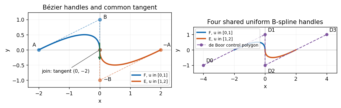
Two quadratic pieces, their Bézier handles, the shared uniform B-spline control polygon, and the vertical tangent at the join
. Details. 
The join has matching positions and first derivatives:Because both pieces have unit parameter intervals, these are also the one-sided derivatives of at . Thus has first-order parametric continuity, and hence first-order geometric continuity, with no corner or cusp. Its nonzero tangent vector points vertically downward.
The second derivatives do not agree:So this is but not parametric continuity. The signed planar curvature has one-sided valuesThe unsigned curvatures agree, but the bending switches sides; there is no second-order geometric continuity through a regular orientation-preserving reparametrization. The join is a reversal of bending with a curvature jump, rather than a smooth zero-curvature inflection.
For the “gradient” compute away from the join:HenceThe zero horizontal derivative is not a stationary point of the parametric curve, since its vertical derivative is . It means that the locally regular curve has a vertical tangent line and cannot have a finite graph derivative as there.
Articles by others on the same topic
There are currently no matching articles.