The square-root reduction of a quadratic eikonal equation explains why two initial normal derivatives are possible. Set . Charpit's equations are , , , , . Parametrize the initial semicircle by , . Tangential compatibility gives , and gives . Thus there are two normal-gradient choices, , , .
Integration gives the requested parametric solutionsFor , , so on the whole right half-plane. For , before focusing at the origin, , so on , . The origin is a caustic for this inward family. The circle is approached only as characteristic time tends to negative infinity, where and its gradient vanish. It cannot be crossed by this initial characteristic chart. Thus the initial data alone permit two branches; each is locally unique only after its normal-gradient sign is chosen.
On the added half-line write , , . Tangential differentiation gives and , . Its characteristics giveThe plus branch is on ; the minus branch is on . On the positive -axis, the semicircle traces are and , respectively. Therefore only matching sign choices are continuous throughout their common positive-axis coverage. Mixed choices agree merely at the initial junction .
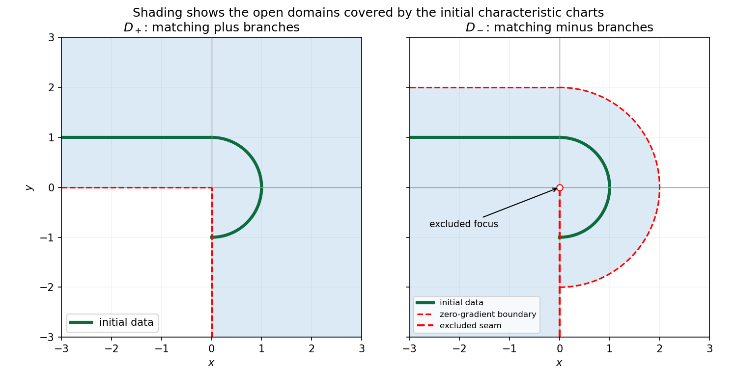
For the matching-plus branch the data-covered open domain isFor the matching-minus branch it isIts formula is in the right portion and in the left portion. The origin is excluded. The negative -axis must also be a cut: the two formulas have different traces there, so including it would destroy continuity. Both matching solutions are across the included positive-axis seam; generally their second transverse derivatives differ, which is compatible with this first-order problem. Values beyond these characteristic charts can sometimes be continued, but are not selected by the initial data through a nonsingular characteristic graph.

With invertible, write the system as , . Real distinct eigenvalues of give strict hyperbolicity; a real complete eigenbasis gives the usual diagonalizable hyperbolic form. The characteristic curves satisfy . Left eigenvectors form characteristic dependent combinations ; for constant coefficients they obey separate transport equations. Characteristic coordinates are functions constant on those curves, such as in the constant case. For variable coefficients extra derivatives of the eigenvectors can couple the combinations; local characteristic directions still follow the real matrix pencil. If is singular one first chooses a noncharacteristic coordinate direction with an invertible coefficient combination.
For the specified constants,Its speeds are and , with left eigenvectors and . HenceThe transported Riemann invariants are , constant on and , respectively. Initial data give and , soInvert these two combinations:Both characteristic feet must lie on the supplied positive initial half-line. ThusOutside this sector at least one invariant needs unsupplied initial data. The closed expressions give one possible extension there but are not uniquely forced by the question's initial half-line.
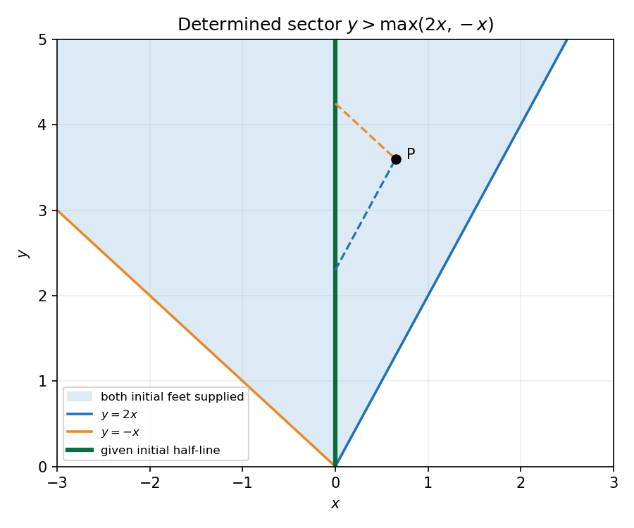
Sector where both backward characteristic families meet the given initial half-line
. Details. 
For fixed source , define the Dirichlet Green function by in , on . It is harmonic away from the source and has singularity . The outward normal vector derivative is at a boundary point of arc-length parameter .
Green's second identity gives . Substituting the two PDEs and the boundary data yieldsThe singular version follows by excising a small source disk and taking its radius to zero, or directly by the distributional identity.
For the upper half-plane use the opposite-sign image source at :The image lies outside the domain, so it is harmonic inside; the true source has the required unit singularity, and the two distances agree at , giving zero boundary value. On that boundary , soThe assumed far-field decay makes the large semicircle contribution vanish. With , the representation becomesFinally set , . The Jacobian matrix cancels the denominator, givingIf is even, the substitution in the Poisson integral gives . At this agrees with the continuous even boundary trace.
At a positive interior maximum, , , and if the point is compared with its past. The PDE instead gives , a contradiction. Thus a positive global/past-strip maximum must come from the spatial boundary or initial-time limit. The far value is positive, so any attained global maximum is positive; the argument does not prohibit a negative local maximum in isolation.
For uniqueness put . It satisfiesThe parabolic comparison principle with zero difference data gives and then , hence . As usual on this noncompact singular-time domain, this uses an admissible comparison class in which the initial and far-field limits justify truncation; for example bounded/subquadratic differences on finite past strips with the corresponding uniform zero traces suffice. A barrier controls spatial infinity, since applied to it is nonnegative. The printed fixed-point limits alone should not silently be substituted for all uniform/growth hypotheses of this comparison argument.
Use drift cancellation in a parabolic similarity reduction. For the similarity ansatz, derivative scaling givesThus , the drift terms cancel, and with . Use the positive-equilibrium separatrix for a cubic profile equation. Multiply by and use the limiting equilibrium to determine the integration constant:The branch approaching the positive far equilibrium satisfies ; the constant equilibrium is included as well. Separation givesFor a finite boundary value at and no interior pole, take . Values describe the corresponding coth-type approach from above; is constant, and positive gives the tanh-type branch. The other first-integral sign cannot approach the positive equilibrium nontrivially as .
Articles by others on the same topic
There are currently no matching articles.