For antiplane shear, the displacement field is , independent of . Its divergence is zero. Consequently the only possibly nonzero components of the stress tensor are the shear stressesThe and components of the Navier-Cauchy equation vanish identically. Its component gives . Each material has constant shear modulus and mass density, so the required wave equation and wave speeds are
At a perfectly bonded elastic interface, both the displacement field and the traction are continuous. Using the same normal on both sides, the only nonzero traction component is . Thus the interface boundary conditions areContinuity of “stress” here means continuity of traction; it does not require equality of the full stress tensors. The rigid plate supplies the remaining boundary condition .
Substitution of the proposed normal mode into the wave equation gives the ordinary differential equationsA nonzero exterior displacement field has exponential decay at infinity only when . Withits wave amplitude is . At the exterior wave amplitude is affine and cannot decay; at it is oscillatory and cannot decay. Setting the exterior wave amplitude identically zero would impose both and , forcing the entire normal mode to vanish.
We also need . Indeed, if , the rigid boundary condition gives with . At the interface,which contradicts continuity of traction because both values of the shear modulus are positive. At , the layer wave amplitude is and the same contradiction follows from .
Therefore . Define the positive transverse wavenumberThe rigid boundary condition now gives . The interface boundary conditions giveNeither nor can vanish for a nontrivial normal mode with . Dividing therefore gives the rigid-backed shear-wave dispersion relation:Conversely, positive satisfying these relations generate a nonzero normal mode through the wave amplitudes above. Its physical displacement field is the real part of the complex expression.
Eliminating the phase velocity from the first two relations yieldsWith , putThen . The dispersion relation becomesHere follows from . The parameter has dimensions of length; and are dimensionless.
For the strict mode count for a rigid-backed elastic layer, considerThe right side is negative, so intersections occur only on the negative branches of the tangent,On each such branch is strictly increasing. If , its limit at is negative infinity. At the other end of the available interval, it is positive: either with , or with . The intermediate value theorem and strict monotonicity give exactly one intersection. No such interval exists when .
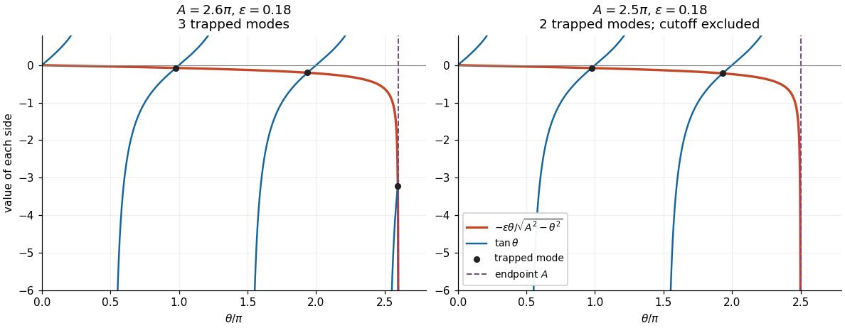
Intersections of the negative tangent branches with the interface loading curve. A branch beginning exactly at the cutoff contributes no trapped mode.
Details. 
Thus the exact answer, including all cutoff values, isAway from , this equals the printed floor function expression . At , the printed expression is one too large: the th interval is empty and the limiting state has , contradicting exponential decay. This exception is present in the native paper, rather than introduced by transcription.
Now hold fixed and let . Neglecting the right side gives and hence the candidate phase velocitiesThe zero is excluded: it would require , already ruled out. For every , the candidate is a valid leading asymptotic expansion. A first correction, obtained by expanding the tangent about , isThe big O notation here assumes a fixed positive gap between and . In particular, when , all leading approximations are valid. The phase velocity increases strictly with , so only the last branch can cause an endpoint difficulty.
If , the formal last equation root lies outside the allowed interval. The actual last equation root approaches , where the small factor is balanced by the vanishing denominator. This is a singular perturbation. For fixed strictly inside that interval, write . Since ,The valid endpoint approximation for a rigid-backed shear mode consequently givesHere we used and . Thus this normal mode approaches the upper wave speed from below; it does not approach the inadmissible value obtained from .
There is a further exceptional fixed value . Put again. Now , so the balance changes toIn the last formula the bracket specifies the first nonzero correction. The zeroth-order candidate is correct as a limit but misses this correction and the positive exterior exponential decay rate. More generally, close to , let and . For , a transition approximation valid on both sides isIt recovers the balance at and the ordinary expansion above the transition. The fixed-endpoint formula involving should be used when is below, and bounded away from, .
Articles by others on the same topic
There are currently no matching articles.