Original solutions to every part of the elasticity and plasticity course of the University of Oxford Part C examination, held on 30 May 2023. Source: released examination PDF, bundle pages 317–320; paper pages 1–4. Numbering follows the original paper. In Question 1(c), the printed count needs a strict-cutoff qualification: at the newly counted state has no exterior exponential decay and must be excluded. The solution includes that correction and the exceptional small-parameter balances. In Question 3(d), purely elastic unloading is valid only until reverse yielding begins.
For antiplane shear, the displacement field is , independent of . Its divergence is zero. Consequently the only possibly nonzero components of the stress tensor are the shear stressesThe and components of the Navier-Cauchy equation vanish identically. Its component gives . Each material has constant shear modulus and mass density, so the required wave equation and wave speeds are
At a perfectly bonded elastic interface, both the displacement field and the traction are continuous. Using the same normal on both sides, the only nonzero traction component is . Thus the interface boundary conditions areContinuity of “stress” here means continuity of traction; it does not require equality of the full stress tensors. The rigid plate supplies the remaining boundary condition .
Substitution of the proposed normal mode into the wave equation gives the ordinary differential equationsA nonzero exterior displacement field has exponential decay at infinity only when . Withits wave amplitude is . At the exterior wave amplitude is affine and cannot decay; at it is oscillatory and cannot decay. Setting the exterior wave amplitude identically zero would impose both and , forcing the entire normal mode to vanish.
We also need . Indeed, if , the rigid boundary condition gives with . At the interface,which contradicts continuity of traction because both values of the shear modulus are positive. At , the layer wave amplitude is and the same contradiction follows from .
Therefore . Define the positive transverse wavenumberThe rigid boundary condition now gives . The interface boundary conditions giveNeither nor can vanish for a nontrivial normal mode with . Dividing therefore gives the rigid-backed shear-wave dispersion relation:Conversely, positive satisfying these relations generate a nonzero normal mode through the wave amplitudes above. Its physical displacement field is the real part of the complex expression.
Eliminating the phase velocity from the first two relations yieldsWith , putThen . The dispersion relation becomesHere follows from . The parameter has dimensions of length; and are dimensionless.
For the strict mode count for a rigid-backed elastic layer, considerThe right side is negative, so intersections occur only on the negative branches of the tangent,On each such branch is strictly increasing. If , its limit at is negative infinity. At the other end of the available interval, it is positive: either with , or with . The intermediate value theorem and strict monotonicity give exactly one intersection. No such interval exists when .
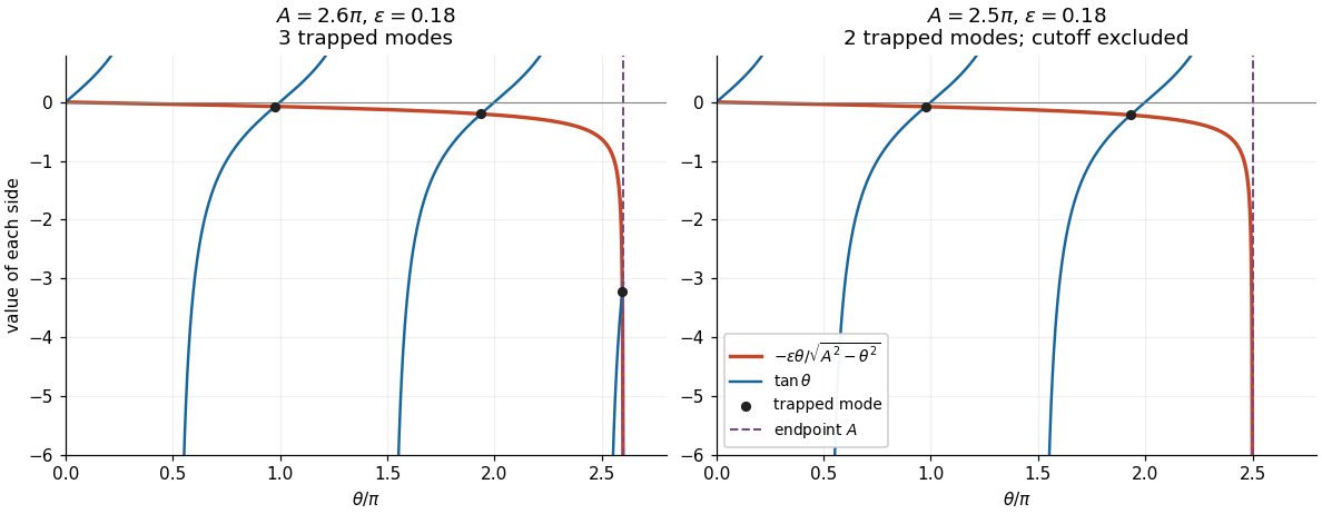
Intersections of the negative tangent branches with the interface loading curve. A branch beginning exactly at the cutoff contributes no trapped mode.
Details. 
Thus the exact answer, including all cutoff values, isAway from , this equals the printed floor function expression . At , the printed expression is one too large: the th interval is empty and the limiting state has , contradicting exponential decay. This exception is present in the native paper, rather than introduced by transcription.
Now hold fixed and let . Neglecting the right side gives and hence the candidate phase velocitiesThe zero is excluded: it would require , already ruled out. For every , the candidate is a valid leading asymptotic expansion. A first correction, obtained by expanding the tangent about , isThe big O notation here assumes a fixed positive gap between and . In particular, when , all leading approximations are valid. The phase velocity increases strictly with , so only the last branch can cause an endpoint difficulty.
If , the formal last equation root lies outside the allowed interval. The actual last equation root approaches , where the small factor is balanced by the vanishing denominator. This is a singular perturbation. For fixed strictly inside that interval, write . Since ,The valid endpoint approximation for a rigid-backed shear mode consequently givesHere we used and . Thus this normal mode approaches the upper wave speed from below; it does not approach the inadmissible value obtained from .
There is a further exceptional fixed value . Put again. Now , so the balance changes toIn the last formula the bracket specifies the first nonzero correction. The zeroth-order candidate is correct as a limit but misses this correction and the positive exterior exponential decay rate. More generally, close to , let and . For , a transition approximation valid on both sides isIt recovers the balance at and the ordinary expansion above the transition. The fixed-endpoint formula involving should be used when is below, and bounded away from, .
Work to first order in the slope and take constant. The elastic beam is slender, its cross-sections remain plane and normal to its centreline, transverse shear deformation is neglected, and the loading is quasi-static. There are no distributed couples. In a non-contact interval the distributed force is and there is no axial distributed force. These are the assumptions of the small-deformation Euler-Bernoulli beam equation, with an optional prescribed tension retained in transverse force balance.
Choose the internal section resultant on the right face of a segment aswhere is the transverse shear force, and take the section bending moment as . Longitudinal and transverse force balance on a segment of length give and . Balancing the torques about its left end gives : the torque from the transverse section resultant is . ThereforeWith this positive- bending moment convention, the linear relation between bending moment and curvature is . Thus , and substitution givesThe tension need not be small compared with the transverse restoring terms, but products arising solely from finite deformation, such as the change of axial extension proportional to , are outside this linear model. A separate axial constitutive constraint would be required to determine an unknown tension from fixed end positions.
In an open contact interval, the upward distributed normal contact force is . At this order the smooth obstacle supplies no axial force; its vertical resultant changes the downward load to . HenceFor nonadhesive unilateral beam contact, the obstacle can push but cannot pull, so . The accompanying constraints are and . A negative would require adhesion and would invalidate the proposed contact region. If is four times differentiable, the distributed normal contact force inside an open contact interval is .
The jump conditions express a connected elastic beam with no concentrated horizontal force or applied couple. Continuity of tension, , follows from horizontal force balance. Continuity of the displacement field and slope, , excludes a break or a kink; a kink would also have unbounded bending elastic energy in this model. Continuity of the bending moment in the absence of a point couple gives , or for constant .
The only allowed discontinuous section resultant is the transverse shear force. Integrating vertical force balance through an upward point force gives . Since , this is preciselyThe same sign follows by integrating , where is the Dirac delta function and the regular terms have vanishing integrals over a shrinking interval. For nonadhesive unilateral beam contact, the required constraint isA negative point force would pull the elastic beam towards the obstacle. At an endpoint where , the third derivative is continuous as well.
With zero tension and zero distributed load, a free interval satisfies . Before contact the entire elastic beam is free, so is a cubic polynomial. The four end boundary conditions determine it uniquely. Reflection preserves those boundary conditions, so the unique solution is an even function and its odd terms vanish. Direct substitution givesFor , its minimum occurs at and is . The constraint is therefore satisfied exactly when . The first contact is at the midpoint:At equality the normal contact force is still zero. The uniqueness used here can also be checked by integrating for the difference of two solutions with homogeneous clamped boundary conditions, which gives and hence .
Seek an even function with isolated contact at . On , the contact and reflection conditions impose and , while the free interval still has . WriteThe two end boundary conditions giveand therefore the full displacement field isThe jump condition at zero gives the upward point forceIt is nonnegative precisely when . In that range . Nonpenetration near zero requires , equivalently . Conversely, when both inequalities hold,with strict inequality away from zero. Thus this is an admissible isolated-contact solution throughoutAt the upper endpoint the contact curvature vanishes, and the profile remains above the obstacle for because . Increasing further would make , forcing penetration near zero. An interval of contact must then develop.
The admissible solution is unique within this linear model: the bending elastic energy is strictly convex on the convex set of admissible profiles with the prescribed end data. Integration by parts shows that a solution with nonnegative contact point forces satisfies the corresponding minimum condition, since every admissible variation lifts a point already on the obstacle. Reflection therefore justifies the assumed even function also after contact.
Let the contact interval be , where . Its slope and curvature vanish. Continuity of the displacement field, slope and bending moment at givesOn the free interval , the cubic polynomial satisfying these three conditions is . Put . The end boundary conditions becomeConsequentlyThis requires , with at the transition. The full displacement field isIt satisfies nonpenetration. In the open contact interval the distributed normal contact force is , since the obstacle is flat and . The normal contact force is concentrated at the two endpoints. At , jumps from zero to ; at , it jumps from to zero. Both upward point forces are thereforeAt they merge into the single midpoint point force of the preceding regime. These formulae belong to the small-slope model; interpreting arbitrarily large as a finite physical rotation would exceed its assumptions.
The net upward force is the sum of the contact point forces, since the distributed normal contact force vanishes in every regime here. Before contact it is zero. During isolated contact it is . For an interval of contact it is , with . ThereforeThe formulae agree at both transitions. At they give , and their first derivatives also agree there. As a check on the sign and normalization, integrating the Euler-Bernoulli beam equation over the whole elastic beam gives , which yields the same values.
Assume homogeneous Lamé parameters, with and positive bulk modulus . For spherical symmetry, write and . Radial force balance is . The given linear elasticity relations implySubstitution into radial force balance givesThusThe volumetric strain is , and the trace of the stress tensor isSince is constant, . The radial elastic compatibility condition follows:This condition is local to a region governed by homogeneous linear elasticity; it is not a constitutive condition for a plastically deforming region.
In the completely elastic exterior, radial elastic compatibility makes constant. The far-field stress vanishes, so and . Radial force balance then gives , whence . The pressure boundary condition is : positive applied pressure is compressive. ThereforeFor completeness, the corresponding radial displacement field is , which gives these components through Hooke's law and decays at infinity.
The Tresca yield criterion becomesFor this is largest at the cavity wall and decreases strictly with radius when . The first yield point is therefore at , where . HenceThe normalization matters: in this paper is a shear yield stress, rather than the uniaxial yield strength.
During increasing pressure, the elastic solution reaches the Tresca yield criterion with . In the plastic shell of a material with perfect plasticity, this sign is retained andRadial force balance becomes . Integrating from the cavity wall, where , givesOutside the plastic shell, radial elastic compatibility and vanishing far-field stress again give and . At the advancing plastic front , the Tresca yield criterion gives , so . Continuity of radial traction now givesThusThe complete stress field of this spherical elastoplastic cavity isAt , the tangential stress also matches because . Outside , the function in the Tresca yield criterion is , which verifies that the remaining material is elastic. As , and the solution joins the entirely elastic regime. The radius is the fixed reference radius of the small-strain model used by the paper.
LetAt maximum pressure, the stress is the field from part (c) with and . Under the assumed elastic unloading, previously accumulated plastic strain is frozen. Therefore it is the stress increment, rather than the total stress, that satisfies homogeneous linear elasticity and radial elastic compatibility. Applying the superposition principle, a pressure change produces the elastic incrementsThey have zero far-field stress and change the wall traction from to . These increments are the same in the formerly plastic and formerly elastic regions because their elastic Lamé parameters agree. Adding them to the maximum-load field givesandThese formulae retain : it records the plastic loading history and is not the instantaneous loading-front formula with substituted for . If the entire return is elastic, setting gives the residual stress after removal of the applied pressure.
To check admissibility, examine the signed difference of the principal stresses in the formerly plastic shell:It immediately moves into the interior of the Tresca yield criterion when unloading starts. It can next reach the opposite limit . For fixed , is largest at and stays above . At the wall,There is no earlier violation in the outer region. Indeed,so its magnitude is no larger than , which has already been controlled by the shell calculation. Hence the first reverse yielding occurs at the cavity wall, withIf , the stress stays within the yield surface throughout unloading to zero. If , it reaches reverse yield exactly at ; further unloading would produce reverse plastic deformation. If , reverse plastic deformation starts while the applied pressure is still positive. ThusIf “yield again while unloaded” includes first touching the yield surface at the final endpoint, the corresponding condition is . The displayed elastic unloading fields are physically valid only for ; beyond that interval a new reverse-plastic region must be solved for. Continuing the elastic formula to when would violate the given Tresca yield criterion.
Articles by others on the same topic
There are currently no matching articles.