Original solutions to examinations of the elasticity and plasticity course of the University of Oxford, using antiplane shear, unilateral beam contact and perfect plasticity.
Original solutions to every part of the elasticity and plasticity course of the University of Oxford Part C examination, held on 30 May 2023. Source: released examination PDF, bundle pages 317–320; paper pages 1–4. Numbering follows the original paper. In Question 1(c), the printed count needs a strict-cutoff qualification: at the newly counted state has no exterior exponential decay and must be excluded. The solution includes that correction and the exceptional small-parameter balances. In Question 3(d), purely elastic unloading is valid only until reverse yielding begins.
For antiplane shear, the displacement field is , independent of . Its divergence is zero. Consequently the only possibly nonzero components of the stress tensor are the shear stressesThe and components of the Navier-Cauchy equation vanish identically. Its component gives . Each material has constant shear modulus and mass density, so the required wave equation and wave speeds are
At a perfectly bonded elastic interface, both the displacement field and the traction are continuous. Using the same normal on both sides, the only nonzero traction component is . Thus the interface boundary conditions areContinuity of “stress” here means continuity of traction; it does not require equality of the full stress tensors. The rigid plate supplies the remaining boundary condition .
Substitution of the proposed normal mode into the wave equation gives the ordinary differential equationsA nonzero exterior displacement field has exponential decay at infinity only when . Withits wave amplitude is . At the exterior wave amplitude is affine and cannot decay; at it is oscillatory and cannot decay. Setting the exterior wave amplitude identically zero would impose both and , forcing the entire normal mode to vanish.
We also need . Indeed, if , the rigid boundary condition gives with . At the interface,which contradicts continuity of traction because both values of the shear modulus are positive. At , the layer wave amplitude is and the same contradiction follows from .
Therefore . Define the positive transverse wavenumberThe rigid boundary condition now gives . The interface boundary conditions giveNeither nor can vanish for a nontrivial normal mode with . Dividing therefore gives the rigid-backed shear-wave dispersion relation:Conversely, positive satisfying these relations generate a nonzero normal mode through the wave amplitudes above. Its physical displacement field is the real part of the complex expression.
Eliminating the phase velocity from the first two relations yieldsWith , putThen . The dispersion relation becomesHere follows from . The parameter has dimensions of length; and are dimensionless.
For the strict mode count for a rigid-backed elastic layer, considerThe right side is negative, so intersections occur only on the negative branches of the tangent,On each such branch is strictly increasing. If , its limit at is negative infinity. At the other end of the available interval, it is positive: either with , or with . The intermediate value theorem and strict monotonicity give exactly one intersection. No such interval exists when .
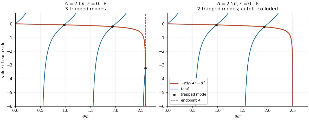
Intersections of the negative tangent branches with the interface loading curve. A branch beginning exactly at the cutoff contributes no trapped mode.
Details. 
Thus the exact answer, including all cutoff values, isAway from , this equals the printed floor function expression . At , the printed expression is one too large: the th interval is empty and the limiting state has , contradicting exponential decay. This exception is present in the native paper, rather than introduced by transcription.
Now hold fixed and let . Neglecting the right side gives and hence the candidate phase velocitiesThe zero is excluded: it would require , already ruled out. For every , the candidate is a valid leading asymptotic expansion. A first correction, obtained by expanding the tangent about , isThe big O notation here assumes a fixed positive gap between and . In particular, when , all leading approximations are valid. The phase velocity increases strictly with , so only the last branch can cause an endpoint difficulty.
If , the formal last equation root lies outside the allowed interval. The actual last equation root approaches , where the small factor is balanced by the vanishing denominator. This is a singular perturbation. For fixed strictly inside that interval, write . Since ,The valid endpoint approximation for a rigid-backed shear mode consequently givesHere we used and . Thus this normal mode approaches the upper wave speed from below; it does not approach the inadmissible value obtained from .
There is a further exceptional fixed value . Put again. Now , so the balance changes toIn the last formula the bracket specifies the first nonzero correction. The zeroth-order candidate is correct as a limit but misses this correction and the positive exterior exponential decay rate. More generally, close to , let and . For , a transition approximation valid on both sides isIt recovers the balance at and the ordinary expansion above the transition. The fixed-endpoint formula involving should be used when is below, and bounded away from, .
Work to first order in the slope and take constant. The elastic beam is slender, its cross-sections remain plane and normal to its centreline, transverse shear deformation is neglected, and the loading is quasi-static. There are no distributed couples. In a non-contact interval the distributed force is and there is no axial distributed force. These are the assumptions of the small-deformation Euler-Bernoulli beam equation, with an optional prescribed tension retained in transverse force balance.
Choose the internal section resultant on the right face of a segment aswhere is the transverse shear force, and take the section bending moment as . Longitudinal and transverse force balance on a segment of length give and . Balancing the torques about its left end gives : the torque from the transverse section resultant is . ThereforeWith this positive- bending moment convention, the linear relation between bending moment and curvature is . Thus , and substitution givesThe tension need not be small compared with the transverse restoring terms, but products arising solely from finite deformation, such as the change of axial extension proportional to , are outside this linear model. A separate axial constitutive constraint would be required to determine an unknown tension from fixed end positions.
In an open contact interval, the upward distributed normal contact force is . At this order the smooth obstacle supplies no axial force; its vertical resultant changes the downward load to . HenceFor nonadhesive unilateral beam contact, the obstacle can push but cannot pull, so . The accompanying constraints are and . A negative would require adhesion and would invalidate the proposed contact region. If is four times differentiable, the distributed normal contact force inside an open contact interval is .
The jump conditions express a connected elastic beam with no concentrated horizontal force or applied couple. Continuity of tension, , follows from horizontal force balance. Continuity of the displacement field and slope, , excludes a break or a kink; a kink would also have unbounded bending elastic energy in this model. Continuity of the bending moment in the absence of a point couple gives , or for constant .
The only allowed discontinuous section resultant is the transverse shear force. Integrating vertical force balance through an upward point force gives . Since , this is preciselyThe same sign follows by integrating , where is the Dirac delta function and the regular terms have vanishing integrals over a shrinking interval. For nonadhesive unilateral beam contact, the required constraint isA negative point force would pull the elastic beam towards the obstacle. At an endpoint where , the third derivative is continuous as well.
With zero tension and zero distributed load, a free interval satisfies . Before contact the entire elastic beam is free, so is a cubic polynomial. The four end boundary conditions determine it uniquely. Reflection preserves those boundary conditions, so the unique solution is an even function and its odd terms vanish. Direct substitution givesFor , its minimum occurs at and is . The constraint is therefore satisfied exactly when . The first contact is at the midpoint:At equality the normal contact force is still zero. The uniqueness used here can also be checked by integrating for the difference of two solutions with homogeneous clamped boundary conditions, which gives and hence .
Seek an even function with isolated contact at . On , the contact and reflection conditions impose and , while the free interval still has . WriteThe two end boundary conditions giveand therefore the full displacement field isThe jump condition at zero gives the upward point forceIt is nonnegative precisely when . In that range . Nonpenetration near zero requires , equivalently . Conversely, when both inequalities hold,with strict inequality away from zero. Thus this is an admissible isolated-contact solution throughoutAt the upper endpoint the contact curvature vanishes, and the profile remains above the obstacle for because . Increasing further would make , forcing penetration near zero. An interval of contact must then develop.
The admissible solution is unique within this linear model: the bending elastic energy is strictly convex on the convex set of admissible profiles with the prescribed end data. Integration by parts shows that a solution with nonnegative contact point forces satisfies the corresponding minimum condition, since every admissible variation lifts a point already on the obstacle. Reflection therefore justifies the assumed even function also after contact.
Let the contact interval be , where . Its slope and curvature vanish. Continuity of the displacement field, slope and bending moment at givesOn the free interval , the cubic polynomial satisfying these three conditions is . Put . The end boundary conditions becomeConsequentlyThis requires , with at the transition. The full displacement field isIt satisfies nonpenetration. In the open contact interval the distributed normal contact force is , since the obstacle is flat and . The normal contact force is concentrated at the two endpoints. At , jumps from zero to ; at , it jumps from to zero. Both upward point forces are thereforeAt they merge into the single midpoint point force of the preceding regime. These formulae belong to the small-slope model; interpreting arbitrarily large as a finite physical rotation would exceed its assumptions.
The net upward force is the sum of the contact point forces, since the distributed normal contact force vanishes in every regime here. Before contact it is zero. During isolated contact it is . For an interval of contact it is , with . ThereforeThe formulae agree at both transitions. At they give , and their first derivatives also agree there. As a check on the sign and normalization, integrating the Euler-Bernoulli beam equation over the whole elastic beam gives , which yields the same values.
Assume homogeneous Lamé parameters, with and positive bulk modulus . For spherical symmetry, write and . Radial force balance is . The given linear elasticity relations implySubstitution into radial force balance givesThusThe volumetric strain is , and the trace of the stress tensor isSince is constant, . The radial elastic compatibility condition follows:This condition is local to a region governed by homogeneous linear elasticity; it is not a constitutive condition for a plastically deforming region.
In the completely elastic exterior, radial elastic compatibility makes constant. The far-field stress vanishes, so and . Radial force balance then gives , whence . The pressure boundary condition is : positive applied pressure is compressive. ThereforeFor completeness, the corresponding radial displacement field is , which gives these components through Hooke's law and decays at infinity.
The Tresca yield criterion becomesFor this is largest at the cavity wall and decreases strictly with radius when . The first yield point is therefore at , where . HenceThe normalization matters: in this paper is a shear yield stress, rather than the uniaxial yield strength.
During increasing pressure, the elastic solution reaches the Tresca yield criterion with . In the plastic shell of a material with perfect plasticity, this sign is retained andRadial force balance becomes . Integrating from the cavity wall, where , givesOutside the plastic shell, radial elastic compatibility and vanishing far-field stress again give and . At the advancing plastic front , the Tresca yield criterion gives , so . Continuity of radial traction now givesThusThe complete stress field of this spherical elastoplastic cavity isAt , the tangential stress also matches because . Outside , the function in the Tresca yield criterion is , which verifies that the remaining material is elastic. As , and the solution joins the entirely elastic regime. The radius is the fixed reference radius of the small-strain model used by the paper.
LetAt maximum pressure, the stress is the field from part (c) with and . Under the assumed elastic unloading, previously accumulated plastic strain is frozen. Therefore it is the stress increment, rather than the total stress, that satisfies homogeneous linear elasticity and radial elastic compatibility. Applying the superposition principle, a pressure change produces the elastic incrementsThey have zero far-field stress and change the wall traction from to . These increments are the same in the formerly plastic and formerly elastic regions because their elastic Lamé parameters agree. Adding them to the maximum-load field givesandThese formulae retain : it records the plastic loading history and is not the instantaneous loading-front formula with substituted for . If the entire return is elastic, setting gives the residual stress after removal of the applied pressure.
To check admissibility, examine the signed difference of the principal stresses in the formerly plastic shell:It immediately moves into the interior of the Tresca yield criterion when unloading starts. It can next reach the opposite limit . For fixed , is largest at and stays above . At the wall,There is no earlier violation in the outer region. Indeed,so its magnitude is no larger than , which has already been controlled by the shell calculation. Hence the first reverse yielding occurs at the cavity wall, withIf , the stress stays within the yield surface throughout unloading to zero. If , it reaches reverse yield exactly at ; further unloading would produce reverse plastic deformation. If , reverse plastic deformation starts while the applied pressure is still positive. ThusIf “yield again while unloaded” includes first touching the yield surface at the final endpoint, the corresponding condition is . The displayed elastic unloading fields are physically valid only for ; beyond that interval a new reverse-plastic region must be solved for. Continuing the elastic formula to when would violate the given Tresca yield criterion.
Source release: Oxford examination archive release thread, Part C bundle pages 430–433. The cover cross-lists Mathematics and Mathematics and Statistics, both at Part C, Wednesday 8 June 2011, 2.30pm–4.00pm.
Answer availability checked on 28 October 2026: bounded official Oxford searches by exact year, course, module and formal code found no exact-paper answers advertised. The official contemporary Part C course document confirms the course identity; it does not advertise answers to this paper. No later-year answer-release policy was assumed to cover 2011.
The deformation gradient is the derivative of the deformation map with respect to the reference configuration coordinates, at fixed time:Its determinant is the local ratio of current to reference volume: for an orientation-preserving deformation in continuum mechanics. Thus elastic incompressibility is the pointwise constraint , rather than a requirement that each individual principal stretch be one.
Choose the outward unit normal to the boundary of the chosen current material subbody. The traction is the contact force exerted on that subbody per unit current area at the boundary point. Reversing the subbody side reverses and .
By Cauchy's stress theorem, the dependence on is linear. With the usual column-vector convention the Cauchy stress tensor satisfiesThe same point has different traction vectors on differently oriented planes, but a single Cauchy stress tensor encodes all of them. In the absence of body couples, conservation of angular momentum makes symmetric.
In the current configuration, balance of linear momentum is the Cauchy momentum equationHere is the Cauchy stress tensor, is current mass density, is body force per unit mass, and is the velocity of the material particle currently at . The expression in parentheses is the material acceleration. The divergence is taken in current spatial coordinates, with .
Equivalently the right side is evaluated at the particle, because this is the same material acceleration in Lagrangian coordinates. For the subsequent static inflation with negligible body force, the equation reduces to .
Write for the reference outer radius and for the current outer radius. The inner material normal is . A fluid pressure applies traction there, so the radial Cauchy stress tensor component must be negative:The second condition uses zero external gauge pressure. Both faces also have zero shear traction; the axisymmetric diagonal stress field satisfies those conditions automatically. The axial constraint is plane strain, so supports may supply an axial reaction; it does not imply zero axial stress.
For the axisymmetric deformation map, take , , and . A reference cylindrical shell of unit axial length has volume , and the corresponding current shell has volume . Elastic incompressibility therefore gives .
Integrating from the inner surface, where , gives . The positive radius is consequentlyThe outer surface is not an additional independent unknown: , and hence .
Use orthonormal cylindrical bases in the reference configuration and current configuration. The deformation gradient maps a radial increment to , an azimuthal arc to , and an axial increment to itself. ThereforeDifferentiating the radius relation gives . Its three principal stretches areTheir product is one, as required by elastic incompressibility. The symbols called “strains” in the source are these stretch ratios; engineering strain would instead subtract one. The axial stretch is one because this is plane strain.
The multiplier enforcing elastic incompressibility contributes an arbitrary hydrostatic stress. Denote it by to distinguish it from the applied pressure . For the neo-Hookean solid, the Cauchy stress tensor is . Thus its principal components areThe axial component is , despite the unit axial stretch. The quantity is a Lagrange multiplier determined together with equilibrium and the traction conditions; it is not obtained by differentiating the reduced stretch energy while ignoring its constraint.
The radial equilibrium equation gives . Set , so that . Substitution of the neo-Hookean solid stress difference eliminates both and :This is a first-order ordinary differential equation for the radial stress, parametrized by the unknown inner radius. For inflation , its right side is positive, so increases from the negative inner pressure to zero at the outer surface. The denominator stays positive because .
Integrate the radial equilibrium equation across the thickness, retaining the integral rather than evaluating its antiderivative. The traction conditions give . Hence must satisfyAll endpoints and coefficients here depend only on and the specified material and reference geometry. This is the required implicit pressure–radius relation for inflation and extension of an incompressible tube with unit axial stretch. In particular gives zero integrand and . Once an admissible root is selected, the radial stress follows by integrating from the outer face, , and the remaining stress components follow from the constitutive equation.
Substituting the sinusoidal plane wave into the Navier-Cauchy equation gives , , and because . Equality of the amplitudes is thereforeThis is an eigenvalue problem for the acoustic tensor . Choosing a nonzero amplitude parallel to gives ; choosing any nonzero amplitude perpendicular to gives . For positive mass density and stable Lamé parameters, both squared speeds are positive. These choices construct nonzero solutions explicitly, proving existence.
Resolve each amplitude by the orthogonal projectionsThe acoustic tensor acts by on the longitudinal line and by on its perpendicular plane. ThusThe longitudinal component is a longitudinal wave, while the two independent transverse polarizations are transverse waves. Each projection obeys its own wave equation, and superposition adds the corresponding solutions.
A general planar disturbance is therefore a sum of the two types. For a single sinusoid with a common speed, both projections cannot be nonzero unless the two speeds coincide: projecting the eigenvalue equation gives and . This distinguishes superposition of waves with different speeds from a mixed polarization traveling rigidly at one speed.
Divide the Navier-Cauchy equation by mass density. Since and , it becomesEquivalently, using the vector calculus identity ,The divergence and curl consequently propagate at and , respectively.
Use the complex amplitude and take its real part at the end; the equations are linear with real coefficients. Let , , and . The differential operators on this exponential function are , , and . Substitution givesThe determinant factors asConsequently choose the positive decay rootsThe Rayleigh wave decay exponents must both give strict decay into the half-space. A genuine nonzero Rayleigh wave combines both, as the free-surface equations below also show. Thus requires . In a stable ordinary isotropic solid , so it is slower even than the transverse wave. The roots depend on the candidate speed as well as the material constants and wavenumber; the speed is fixed by the boundary condition.
For the root the elastic wave polarization is parallel to the complex derivative vector , givingFor the root the field has zero divergence, , givingThese relations also follow by inserting each decay root into either row of the matrix. The complete decaying displacement field has complex componentsmultiplied by , followed by the real part. The first constituent is irrotational and the second is divergence-free; both are needed to cancel the two surface tractions.
The material occupies , so its outward unit normal at the surface is . A free surface has zero traction, . ThereforeThe third condition is automatic for the two-dimensional displacement field with zero third component and no dependence on the third coordinate. The first two impose zero shear and normal stress at the free surface.
Write the in-plane displacement field as . The infinitesimal strain tensor gives , , and . The two nontrivial zero-traction conditions becomeEquivalently for the complex amplitudes they are and . Because the constitutive equation is real and linear, vanishing of these complex amplitudes enforces the conditions at every position and time.
Substituting both profiles into the shear traction condition givesFor the normal traction, use and . Removing the common nonzero factors yields the second equation. ThusA nonzero displacement field requires the determinant to vanish:Let and . Cancelling gives the Rayleigh secular equationSquaring and excluding the zero root gives ; any candidate must still satisfy the unsquared equation and the decay inequalities. For stable isotropic elasticity , this cubic has one root in : its values at zero and one have opposite signs, and its strictly negative second derivative on this interval prevents a second crossing back to a positive final value. Both sides of the unsquared equation are positive there, so this root is valid.
The root of the squared equation is not a propagating surface wave: at , the two roots coincide, and the null combination in this representation produces zero displacement field. As a numerical example, gives and . The surface-wave speed is independent of in this homogeneous half-space model.
Let be arc length, so inextensibility makes a unit tangent vector. The curvature is , hence for uniform bending stiffness. Balance of linear momentum in static equilibrium gives a constant resultant .
Taking the cross product directly,The scalar component of conservation of angular momentum therefore becomesTogether with and , this Euler elastica equation determines the centerline once the appropriate boundary conditions are supplied.
Put . With , the Euler elastica equation is . Linearization about the straight configuration gives . Under the boundary conditions explicitly stated, , a nonzero solution requiresThus with only the stated boundary conditions, the first critical compressive force is . The corresponding linear transverse displacement field, with , isand to first order. These are the successive small-amplitude buckling modes. The nonlinear branches retain the simple pendulum equation; if the angular amplitude is and , fitting half-periods into the rod gives , which tends to as . Here is the complete elliptic integral of the first kind, with its modulus, not its squared parameter.
Endpoint position compatibility for the Euler elastica adds a condition when fully fixed clamps have equal transverse height. If the word “clamped” also imposes , then . With , this retains only even , yieldingThe same exclusion is exact on the nonlinear branches: integrating the elastica equation gives , and an odd number of half-periods reverses the nonzero endpoint slope. Hence odd changes the endpoint height. The conventional fixed-clamp first Euler buckling load is the second boxed value, whereas the source's explicitly listed boundary conditions alone give the first. Additional clamped modes with a nonzero transverse reaction require releasing the imposed . Load-controlled buckling also permits axial shortening; an exactly inextensible rod whose endpoint separation is fixed equal to its full length has no room to buckle.
Set . The Euler elastica equation becomes . Multiplying by gives the first integralStraight asymptotic ends require and a horizontal tangent, so . This is the separatrix of a simple pendulum with its angle shifted by . A nonconstant solution moves from to , with the same physical tangent at both ends, taking infinite arc length to approach either limit. One explicit representative isUsing and and integrating gives the tensile elastica loopThis solution is nontrivial, tends to horizontal straight tails, and has finite excess bending energy. It is also necessarily self-intersecting. Indeed is even and is odd. For , let . Near zero , while , so there is a root . At the two distinct parameters , both points have and the same . Numerically .
Any nonconstant smooth solution with the same straight asymptotic conditions has this first integral. Between consecutive horizontal orientations, separating variables gives the displayed solution up to translation, reflection, and reversal. It cannot pass through a straight equilibrium at a finite parameter, by uniqueness of the ordinary differential equation. Thus all such nontrivial branches have the same loop crossing. This is an ideal zero-thickness rod solution; a physical rod with self-contact excluded cannot realize the crossing without adding contact forces.
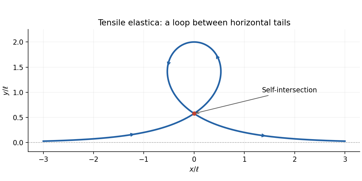
The tensile elastica loop and its self-intersection
. Details. 
Take the clamp at with . An end force without an applied end moment gives the free-end condition . With , the Euler elastica equation is . For , is small, so the leading equation isIntegrating with the two boundary conditions givesTo first order, and . HenceEquivalently at leading order, the familiar cantilever response. Because , the deflection is downward. The free-end displacement field and slope are and . The remainder notation holds with fixed positive and nondimensional unit rod length.
Original solutions to the paper released at the source request. The complete editable transcription is retained in the private examination archive.
The displacement follows a material point from its reference position to its current position:The deformation gradient is the Jacobian matrix , and the volume Jacobian isFor an orientation-preserving physical deformation, measures the local volume expansion factor. Incompressibility requires ; conservation of mass gives . For small displacement gradients, . If a spatial representation is desired, the same displacement is .
A Cartesian Cartesian second-rank tensor has components transforming under a constant orthogonal change of axes asHere and . By the chain rule and orthogonality,Thus the displacement gradient is a Cartesian second-rank tensor. Its symmetric part transforms in the same way:Hence the infinitesimal strain tensor is also second-rank. This is a passive coordinate rotation, under which both reference and spatial coordinates rotate; it does not assert finite-deformation frame indifference of the linearized strain formula.
The traction on the oriented solid element isWith constant Lamé coefficients and derivatives in the reference variables,Substitution into balance of linear momentum givesTo check the vector identity componentwise, contract the two alternating tensors:Rearranging proves . Therefore
Assume . Dotting the decomposition with givesCrossing it on the left by and using gives . ThusIndeed , verifying the decomposition and the imposed transverse condition.
Apply the wave ansatz to the oscillatory displacement about a static body-force balance, or equivalently to the zero-body-force homogeneous equation. The parallel and perpendicular polarizations have speedsThe first is longitudinal and the second transverse. A wave family is dispersive when its phase speed varies with wavenumber. In each of these homogeneous bulk families, , so both are nondispersive and group and phase speeds coincide.
Substitution of givesThe oscillatory seam solution requires , givingFor an exponentially decaying exterior, with , so the same differential equation instead requiresThe printed exterior plus sign is inconsistent with its decaying ansatz and must be a sign error. The guided mode has , so a slower shear-wave seam than its cladding is necessary.
For an even seam mode , upper-interface displacement and traction continuity giveThe lower interface gives the same equations when . Eliminating the amplitudes yieldsFor an odd seam mode , the equations areWith the lower condition agrees, and elimination givesThese interface conditions together with the two corrected dispersion identities determine the guided-wave branches.
In the formal stiff-cladding limit with a nonvanishing exterior decay rate, the interface displacement tends to zero. The even seam mode then has , whereas the odd mode has . The positive wavenumbers areThe zero odd index would give an identically zero mode and is excluded. The smallest even transverse wavenumber is , so its lowest branch satisfiesThis is the symmetric-mode cutoff: the actual limiting branches have the discrete listed values of . If the exterior shear speed remains finite, the separate decay requirement still applies; the cutoff alone does not replace that guided-wave condition.
Differentiate the displacement components. The shear strains involving vanish because and . The full infinitesimal strain tensor isIn particular . Substituting the Lamé coefficients into the constitutive law givesFor example : the thickness-direction strain supplies exactly the plane-stress Poisson correction. Also , confirming the off-diagonal factor.
Contract the tensors, counting both off-diagonal shear terms:Since , integration givesFor the general midplane deflection, expand the energy density as . A variation givesFor clamped variations, on the boundary, so integrating twice transfers all derivatives to without a boundary contribution. The bulk coefficient isStationarity for all compactly supported variations and the fundamental lemma therefore give
Articles were limited to the first 100 out of 175 total.
Articles by others on the same topic
There are currently no matching articles.