Past exam of the general relativity course of the University of Oxford / 2011 (C7.2a, DMAC 2B78)

Source: Mathematics release, bundle Part C 2007 11.pdf, pages 441–444. This Mathematics Part C paper was sat on 16 June 2011, 9.30–11.00am.

The department's answer-release policy excludes ordinary odd years. Exact-code and title checks found no matching answer advertisement. A separate 2011 General Relativity solutions listing links a Physics B3 paper, whose cover and questions do not match this Mathematics paper. All three unpartitioned questions and their individual requests are answered here.

The paper uses $T_{\mu \nu }{}^{\lambda }={\Gamma }_{\nu \mu }{}^{\lambda }-{\Gamma }_{\mu \nu }{}^{\lambda }$, the negative of a common torsion tensor convention. Keep that sign throughout. Also, ${\nabla }_{\mu }{\nabla }_{\nu }\phi$ denotes the covariant Hessian, so the second derivative acts on the lower index $\nu$ of the covector ${\nabla }_{\nu }\phi$; it is not just a composition of two directional derivatives on a scalar.

Since the covariant derivative of a scalar field is its ordinary derivative,Commuting the ordinary partial derivatives therefore givesFor a vector field, write $D_{\nu }{X}^{\lambda }={\partial }_{\nu }{X}^{\lambda }+{\Gamma }_{\nu \rho }{}^{\lambda }{X}^{\rho }$. This is a tensor with one covariant and one contravariant index. HenceSubtracting the expression with $\mu ,\nu$ exchanged, the first two terms combine toThe coefficients of first derivatives of $X$ in those two terms cancel. The last terms give $({\Gamma }_{\nu \mu }{}^{\sigma }-{\Gamma }_{\mu \nu }{}^{\sigma })D_{\sigma }{X}^{\lambda }$. Identifying the curvature coefficient yieldsHere the bracket denotes antisymmetrization of the tensorial second covariant derivative, consistently with the preceding calculation.

To check tensoriality directly, antisymmetrize the supplied transformation law of the connection coefficients in the two lower indices. The inhomogeneous term vanishes because mixed coordinate second derivatives are symmetric. The remaining transformation law iswhich is precisely that of a $(1,2)$ tensor. Intrinsically, with the paper's sign,The derivative terms involving the components of $X,Y$ cancel against their Lie bracket, leaving $({\Gamma }_{\nu \mu }{}^{\lambda }-{\Gamma }_{\mu \nu }{}^{\lambda })X^{\mu }{Y}^{\nu }$. This also shows that the expression is linear over smooth functions in each argument.

Finally take the torsion-free connection and the commuting parameter fields $Y,Z$ along the geodesic family. Vanishing torsion gives ${\nabla }_{Y}Z={\nabla }_{Z}Y$, while affine geodesic parametrization gives ${\nabla }_{Y}Y=0$. The curvature operator in the specified convention isThereforeIn components this is the geodesic deviation equationThe connecting field represents infinitesimal separation within the family, so this is a linear equation for relative free-fall acceleration, rather than an exact coordinate difference for widely separated worldlines.

For this question use the Levi-Civita connection, its metric compatibility and the usual curvature symmetries. In the index ordering of Question 1, put $R_{\mu \nu \rho \sigma }=g_{\sigma \lambda }{R}_{\mu \nu \rho }{}^{\lambda }$ and $R_{\nu \rho }=g^{\mu \sigma }{R}_{\mu \nu \rho \sigma }$. Contract the second Bianchi identity in its derivative index $\mu$ and curvature index $\rho$. The curvature symmetries giveNow contract $\lambda ,\sigma$. The left-hand side becomes $-{\nabla }^{\rho }{R}_{\nu \rho }$, while the right-hand side becomes ${\nabla }^{\sigma }{R}_{\nu \sigma }-{\nabla }_{\nu }R$. ThusUsing $\nabla g=0$ yields the contracted Bianchi identityTaking the covariant divergence of the Einstein field equations, with constant $G$, then gives $8\pi G{\nabla }^{\mu }{T}_{\mu \nu }=0$. The matter equation is therefore consistent with the geometric identity rather than imposing an extra incompatible condition on the metric.

Stress-energy conservation expresses the local balance of energy and momentum, including their transport and the effects of the gravitational Levi-Civita connection. In a freely falling frame at a point it reduces there to the familiar ordinary divergence law. A global conserved energy requires additional geometric structure, such as a timelike Killing vector field; it does not follow in an arbitrary spacetime just by replacing a covariant derivative with an ordinary derivative.

For relativistic dust,With signature $(+,-,-,-)$, $u^{\nu }{u}_{\nu }=1$ implies $u_{\nu }{u}^{\mu }{\nabla }_{\mu }{u}^{\nu }=0$. Contracting gives ${\nabla }_{\mu }(\rho u^{\mu })=0$; where $\rho >0$, substitution then gives $u^{\mu }{\nabla }_{\mu }{u}^{\nu }=0$. Thus the continuity law combines rest-mass conservation and free geodesic motion for this matter model.

For the Newtonian limit, take $c=1$ and $\eta =\mathrm{diag}(1,-1,-1,-1)$, consistently with Question 3. Use the static weak field sourced by the time-independent, slowly moving matter, retaining first order in $ϵ$ and leading order in the spatial speed. Write spatial gradients with ${\partial }^i={\delta }^{ij}{\partial }_j$ here; these are Euclidean spatial indices in the Newtonian equation. The Levi-Civita connection formula givesThe exact change from proper time to $t$ in the spatial geodesic equation isTerms containing spatial velocities are negligible at leading order, leavingAn additive constant in $\Phi$ is immaterial to this acceleration and is normally fixed by the asymptotic time normalization. With units restored, $g_{00}=1+2{\Phi }_{\mathrm{physical}}/c^2$.

At the same order, staticity and the curvature definition giveThe trace of the four-dimensional Einstein equations is $R=-8\pi GT$, so their trace-reversed form isFor nonrelativistic dust, $u^0\simeq 1$, $u^i\simeq 0$, so $T_{00}\simeq \rho$ and $T\simeq \rho$. Keeping leading matter terms therefore gives $R_{00}=4\pi G\rho$. Combining this with the geometric expression yieldsThis trace reversal is essential: equating $R_{00}$ directly to $8\pi G\rho$ would miss the factor of two. The approximation is the quasistatic Newtonian sector; arbitrary independently imposed gravitational radiation is not part of that sector.

Let $f(r)=1-2m/r$ and work in the exterior $r>2m$, with $G=c=1$. The affinely parametrized geodesic Lagrangian isIts polar-angle equation isThe initial data $\theta =\pi /2$, $\dot{\theta }=0$ therefore remain in that plane. Rotational symmetry allows the axes to be chosen so that any nonradial initial trajectory has those data: its conserved angular-momentum direction fixes an orbital plane through the centre. Radial trajectories can also be placed in an equatorial plane.

The coordinates $t,\varphi$ are cyclic in $L$, so their canonical momenta are constant:The corresponding Killing vector fields are ${\partial }_t$ and ${\partial }_{\varphi }$. With the displayed signature, $g({\partial }_t,\dot{x})=E$ and $g({\partial }_{\varphi },\dot{x})=-J$, explaining the sign in the second canonical momentum. Thus $E$ is conserved energy per unit rest mass for a massive particle parametrized by proper time, and $J$ is its axial angular momentum per unit rest mass. For a photon, affine rescaling rescales both constants; after the tangent is normalized to the physical four-momentum they represent its energy at infinity and axial angular momentum. Their ratio $b=J/E$ is the signed impact parameter.

In the equatorial plane, the photon satisfies the null geodesic constraintwhich givesFor $J\ne 0$, put $u=m/r$ and $\alpha =Em/J$. Thenand consequentlyThe $J=0$ radial case is not represented by $\varphi$ as an orbit parameter.

There is a circular photon orbit at $r=3m$, but it is unstable. The radial effective potential isA circular orbit requires $V^{\prime }(r)=0$ and $E^2=V(r)$, givingIts second derivative isIt is a maximum, rather than a minimum, so radial perturbations depart from the orbit. Equivalently the second-order orbit equation is $u^{\prime \prime }=3u^2-u$. Linearizing about $u_c=1/3$ gives $\delta u^{\prime \prime }=\delta u$, with modes $e^{\varphi }$ and $e^{-\varphi }$. The existence of a growing mode directly contradicts the printed stability claim. Exact initial data can remain circular, but that does not make the orbit stable.

The supplied implicit expression describes the critical-energy family with ${\alpha }^2=1/27$, as fixed by the circular orbit. DefineRationalizing once gives $F=(\sqrt{3}-s)/(2(\sqrt{3}+s))$ andDifferentiating $F(u)=A{e}^{\varphi }$ gives $F^{\prime }{u}^{\prime }=F$, soThis verifies the first-order equation for every allowed integration constant $A$ on its real branch. For $A=0$ the derivative argument is replaced by direct substitution: $u=1/3$ is constant and solves the critical equation. The displayed family does not solve the equation at an independently arbitrary value of $\alpha$.

For $A>0$, write $q=A{e}^{\varphi }$. On the physical exterior branch,As $\varphi \to -\infty$, $q\to 0^{+}$ andThus for $A=0$ the photon remains exactly on the circular orbit. For $A>0$ it approaches $r=3m$ from outside through indefinitely many revolutions in the negative-$\varphi$ limit. With increasing $\varphi$, this same branch peels away outward and reaches infinity when $q=1-\sqrt{3}/2$. Reversing the direction of motion gives an incoming critical ray asymptotically approaching the photon circle. These are separatrix trajectories, not evidence of stability.

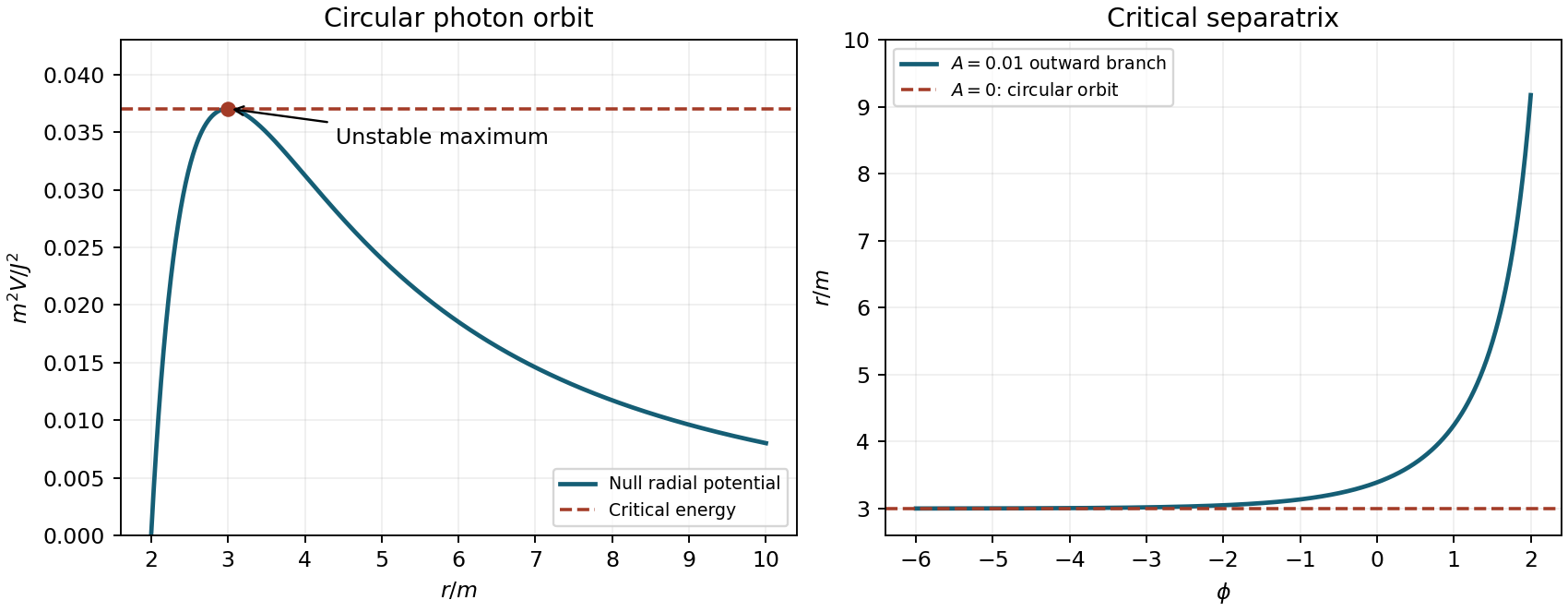
The potential maximum and the outward-growing radial separation display the same instability in two complementary descriptions.