Source bundle pages 139–144. The paper cover establishes 2022; the attachment filename uses 2021.
For the Levi-Civita connection, the all-lowered Riemann curvature tensor has the algebraic symmetriesThe first Bianchi identity is the cyclic identityThese statements concern the Riemann curvature tensor at each point and are unchanged by reversing its overall curvature sign convention.
A semicolon denotes the covariant derivative for the Levi-Civita connection. For example, the four lower indices of the Riemann curvature tensor contribute four connection terms:Here is a partial derivative, are Christoffel symbols, and repeated indices are summed from to . Write for the metric tensor, for its inverse metric, for the Ricci tensor, and for the Ricci scalar. This tensor contraction agrees with the paper's .
By metric compatibility, the inverse metric may pass through each covariant derivative. Contracting the second Bianchi identity with giveswhere is the same covariant derivative as the semicolon. Next contract with . Antisymmetry of the first pair gives , soThus the contracted Bianchi identity is . Raising the remaining index and using metric compatibility provesThe Einstein tensor therefore has identically zero covariant divergence, without imposing any field equation. This makes the Einstein field equations compatible with stress-energy conservation, , where is the stress-energy tensor. The connection terms describe how energy and momentum are compared at neighboring points; ordinary componentwise partial derivatives would not give a coordinate-independent conservation law in curved spacetime.
Take the tensor contraction of the Einstein field equations with the inverse metric . In four-dimensional spacetime, , henceHere is the tensor contraction of the stress-energy tensor. Substituting this result back into the Einstein field equations, while keeping both free indices lowered, gives the trace-reversed stress-energy tensor:The factor uses the dimension four: in dimension , the Trace-reversed Einstein field equations in D dimensions have in place of .
Use and metric signature . With the source's curvature sign convention, the Ricci tensor isIts time-time component is thereforeFor a slowly moving, pressure-negligible source, the stress-energy tensor is approximated by relativistic dust: , where is mass density and is the four-velocity. In its approximate rest local inertial frame, and . Thusand the trace-reversed stress-energy tensor satisfies
Independently, introduce the metric perturbation , with and constant Minkowski metric . The Christoffel symbols are first order in , so their products are discarded in the weak-field approximation. With a comma denoting a partial derivative, the linearized Riemann curvature tensor isTaking the tensor contraction gives, to this order,In the static Newtonian limit, all time partial derivatives vanish. The constant also has zero partial derivatives, leavingHere is the spatial Laplace operator in the approximately Cartesian background coordinates. This sign follows the paper's curvature sign convention.
For the Newtonian gravitational potential , the weak static metric tensor has . The Newtonian limit derived above consequently givesMatching the Poisson equation for Newtonian gravity, , fixesHere is the gravitational constant and is the speed of light. This negative coupling agrees with the source formula sheet. The familiar positive coupling uses the opposite curvature sign convention for the Ricci tensor; the physical Poisson equation for Newtonian gravity is the same.
Choose normal coordinates centered at an event . At , the metric tensor in these coordinates is the constant Minkowski metric , with measured in length units, and its first partial derivatives vanish. In arbitrary coordinates , the chain rule for the line element givessoThis construction is pointwise. At nearby events, the metric tensor in the chosen normal coordinates is , with the quadratic corrections determined by the Riemann curvature tensor. Replacing by one constant Minkowski metric throughout an open region would make that region flat, so it cannot describe general curved spacetime exactly.
For a contravariant vector field , the covariant derivative isThe Levi-Civita connection is the unique torsion-free connection satisfying metric compatibility. Its Christoffel symbols in a coordinate basis areThere is generally no symmetry interchanging the upper index with a lower one. The Christoffel symbols themselves are not the components of a tensor.
An ordinary partial derivative of the components of a vector field includes the apparent change caused by the varying coordinate basis. The connection term corrects for that change, so obeys the tensor component transformation law. It gives coordinate-independent ways to express parallel transport, geodesics and stress-energy conservation in curved spacetime.
Each lower index contributes a minus connection term to the covariant derivative of the metric tensor:Substitute the Christoffel symbols of the Levi-Civita connection and use the inverse metric identity :Adding cancels the first and third terms and leaves exactly . HenceThis is metric compatibility: the Levi-Civita connection preserves the inner product under parallel transport.
The metric tensor in a basis is . Differentiating this inner product with the product rule and using the assumed basis-derivative relation yieldsThus the coefficients satisfy metric compatibility. For a coordinate basis with zero torsion tensor, symmetrizing this relation in , adding the corresponding two equations and subtracting the third givesThey are therefore the Christoffel symbols of the Levi-Civita connection. Metric compatibility by itself does not establish zero torsion tensor; that also uses the coordinate basis and its commuting coordinate derivatives.
For an embedded curved surface, the stated ambient basis-derivative relation needs a qualification: the Gauss formula is , where is a unit normal and is the second fundamental form. The normal term has zero inner product with each tangent basis vector, so the displayed identity for still holds. For a concrete counterexample to dropping that term, on a two-sphere one has , whereas every is zero. Thus the intrinsic connection describes the tangential projection of the ambient derivative.
In standard spherical coordinates, parametrize the two-sphere byThe coordinate basis transforms from the fixed Cartesian basis according to . ThereforeTheir inner products are , and . Thus the induced metric isThe source's intermediate display places an extra outside entries already labelled . Interpreting those entries as the actual metric tensor components would double-count the factor: for example, gives directly from , not . Its final matrix is the correct induced metric; the entries of its intermediate matrix must instead denote dimensionless coefficients.
The only nonconstant entry of the metric tensor is , whose partial derivative is . The nonzero Christoffel symbols areAlong a fixed latitude with , parallel transport givesSet and . Since is fixed, this linear ordinary differential equation becomesIt is a rotation at constant rate . Its general solution, also valid at the equator where the rate is zero, isThe initial data give and . At , a complete circuit has , soThe physical squared length uses the metric tensor, rather than the Euclidean sum of coordinate components:It is constant and equals for these data. More generally, metric compatibility gives . The final change of direction is holonomy, exemplified by parallel transport around a latitude of the unit sphere; parallel transport preserves length without requiring the direction to return unchanged.
A photon follows a null geodesic, whose spatial path approaches straight lines far from the deflecting mass. Extend the incoming asymptote forward: this is the reference path the photon would follow if the mass were removed while its incoming direction and transverse offset were held fixed. The impact parameter is the perpendicular distance from the mass to that incoming asymptote. It is not, in general, the distance of closest approach.
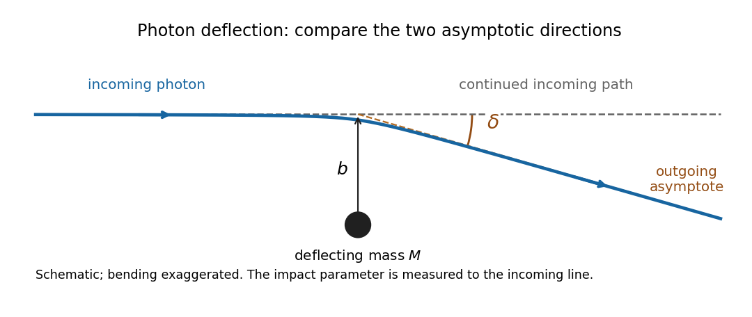
Impact parameter and deflection relative to the continued incoming photon path
. Original schematic, with bending exaggerated. The dashed horizontal line is the undeflected reference path. The outgoing dashed asymptote makes angle delta with it; b is measured to the incoming asymptote, not to the bent ray. Details.
The positive deflection angle is the angle between the outgoing propagation direction and the continued incoming direction. The photon bends toward the mass, so a ray passing above it has a downward outgoing slope in the figure. In the weak-field approximation for an isolated spherical mass, Schwarzschild light deflection gives for distant endpoints. This angle differs from the apparent image angle measured from the observer's line of sight to the mass.
By spherical symmetry, choose the orbital plane to be . The geodesic Lagrangian of the Schwarzschild metric isFor a massive test particle, dots denote proper time derivatives and . The cyclic coordinates and give, through the Euler-Lagrange equations, two constants:At infinity, is the Lorentz factor. The constant is the specific angular momentum, and the energy per unit rest mass is . The normalization of the four-velocity givesUse and define the energy-normalized angular momentum for a Schwarzschild geodesicThenFor an incoming massive test particle with impact parameter , , so . In particular, is not the same as the specific angular momentum unless .
A photon has no proper time parametrization and no finite Lorentz factor. For it, use an affine parameter in the same geodesic Lagrangian and impose . The ratio remains well defined, and the null result isEquivalently this is the ultrarelativistic limit of the massive formula at fixed , with . The printed massive formula needs this interpretation before it is applied to a photon.
Let , , and use a prime for . The null geodesic first integral obtained above becomesDifferentiating with respect to and dividing by away from a turning point givesThe same differential equation holds at the turning point by continuity. When , the general solution is . Choose the angular origin so that the incoming asymptote has and the unperturbed closest approach has . The impact parameter then fixesThis is the straight reference path, not a curved orbit.
For perturbation theory with , write , where . Inserting this into the differential equation and discarding second-order terms givesA particular solution and the complementary solution areChoosing retains reflection symmetry about and the specified impact parameter to first order. The two distant zeros of then occur at and . Their separation exceeds by , consistently giving the Schwarzschild light deflection .
In the thin-lens approximation for gravitational lensing, consider a ray crossing the lens plane at transverse distance above the aligned source-observer axis. With the observer at axial position , the black hole at and the source at , the segment joining the lens plane to the source has slope , while the segment joining the observer to the lens plane has slope . The observer sees the ray at apparent angle to the axis. When following the photon toward the observer, the two small angles to the axis have magnitudes and . The physical bend is their sum:Substitute the Schwarzschild light deflection, , and use :Every azimuth around the axis is equivalent by rotational symmetry. Isotropic emission therefore supplies rays at all these azimuths, and the ideal image is an Einstein ring centered on the black hole, with Einstein angular radius and angular diameter . A finite source size or imperfect alignment broadens or breaks the ideal ring.
The stated expression uses small angles, distant endpoints and weak-field approximation , with ordinary Euclidean distances. For cosmological gravitational lensing, use angular diameter distances in ; generally .
For the hypothetical Hubble flow, Hubble's law gives , where and is the Hubble constant. The accompanying constants sheet is not present in the supplied PDF, so retain its dependence explicitly. Taking as an illustrative input, and using one million parsecs equal to ,A year of days contains . ThereforeEquivalently, gives . This is a counterfactual recession rate for independently comoving bodies, rather than a prediction for the actual Earth-Moon orbit.
The Earth-Moon pair is a gravitationally bound system, so its separation does not obey . The Hubble flow describes the motion of the approximately homogeneous cosmological matter distribution; it is not a compulsory extra velocity assigned to the members of every local orbit. Thus the numerical proximity of the counterfactual rate to is not evidence for that explanation.
The observed recession arises principally from tidal dissipation. The Earth rotates faster than the Moon orbits, so the displaced tidal response transfers angular momentum from the Earth's spin into the lunar orbit. For a nearly circular orbit, increasing orbital angular momentum increases its size. A model of this effect must include the appropriate tidal response, rather than add a universal Hubble flow recession.
A residual local cosmological tidal acceleration can exist, but its background scale is , not an imposed first-order secular drift . At ,using . The cosmological scale is about of the mutual gravitational acceleration. Its detailed coefficient depends on how the local system is embedded in the cosmological background. Cosmological expansion can be neglected for the lunar recession calculation at the stated precision; this conclusion follows from binding and the tiny residual local cosmological tidal acceleration, rather than from comparing two recession speeds.
Let be the initial epoch, let be the physical radius of the outer matter shell, and put . The background Einstein-de Sitter universe has critical density at that epoch. Its mass inside is , where is the actual conserved mass. Hence the background Friedmann equation impliesFor spherical collapse of pressureless matter, with no shell crossing, the shell theorem gives . Its conservation of energy first integral isConsequentlyFor , the initially expanding branch reaches cosmological turnaround at . Since on that branch, the elapsed cosmic time isThis is spherical turnaround from an unperturbed Hubble velocity. The integral measures the comoving matter observers' time interval in the pressureless model. The integration variable is the physical radius, not the radius divided by the background scale factor. If an absolute cosmic time is wanted, add to the displayed interval.
Set , retaining in . Replacing only the lower integration limit by zero givesSubstitution of the constants yieldsTo quantify the approximation, write . The true lower limit is , and an elementary integration by substitution, , givesSince , the approximate time is too large by a relative fraction . This explains why changing the lower limit introduces little error for a small excess mass. The cosmological turnaround time diverges as , consistently with the absence of finite cosmological turnaround in an exactly critical Einstein-de Sitter universe.
There are two first-order effects: an intrinsic temperature change from adiabatic compression, and the gravitational redshift of the emerging photons. Evaluate the excess Newtonian gravitational potential at the boundary of the spherical fluctuation, with the exterior reference potential subtracted:In the weak-field approximation, gravitational time dilation gives . A local emitter's successive wave crests therefore arrive farther apart at a reference observer outside the potential well. Their frequency changes by . Since a redshifted black-body radiation spectrum has its temperature scaled by the same factor as its frequency, the gravitational contribution is
For the intrinsic effect, compare the local scale factor with the unperturbed value at the reference epoch. An equilibrium photon gas has energy density and pressure . For adiabatic compression, the first law of thermodynamics applied to a comoving volume givesThus is constant along this adiabatic process, and the initial intrinsic contribution is . The smaller local expansion associated with the fluctuation leaves its radiation hotter; this is the compression or local expansion-history contribution, distinct from the clock-rate effect on the escaping radiation.
Multiplying the two first-order factors, and cancelling the common subsequent background redshift, givesFor the overdense region produced by adiabatic compression, , so the final term is positive. It competes with the negative gravitational redshift term. Their sum is the intrinsic-plus-endpoint part of the Sachs-Wolfe combination; computing a full observed Cosmic microwave background anisotropy can also require Doppler CMB anisotropy and the Integrated Sachs-Wolfe effect.[ref]
Cosmology by David Tong. Sections 3.4 and 3.4.1, equations (3.210)–(3.212): adiabatic temperature perturbations and gravitational redshift contributions
The paper occupies bundle pages 132–137. Its cover establishes 2021; the attachment filename uses 2020.
In general relativity, gravity is the geometry of spacetime, whose curvature is related to the stress-energy tensor, and freely falling test particles follow timelike geodesics of its metric tensor.
The apple's proper time is the time read by a clock carried with it, with for metric signature . At any event choose a local inertial frame with coordinates , in which free motion satisfies at that event. The chain rule givesMultiplying by the inverse coordinate Jacobian matrix yields the exact geodesic equationHere are the observer's coordinates, is the apple's four-velocity, and the Christoffel symbols describe the Levi-Civita connection. The last expression applies when the coordinates are locally inertial at the event considered; one such chart need not remain inertial throughout a finite region.
Choose , so . In the weak-field approximation and at small spatial speed compared with , the leading spatial geodesic equation isIt is exact at the release event when all spatial vanish, and is the intended approximation to the displayed expression in the source. Terms and cannot generally be dropped; the time component must also be retained to find changing . For a concrete counterexample to the unrestricted expression, a straight free trajectory , in flat spacetime has polar radius and , although . The missing angular term supplies that radial coordinate acceleration.
Approximate Earth by an isolated, nonrotating, spherically symmetric body. By Birkhoff's theorem, the exterior vacuum metric tensor is the Schwarzschild metric. With it isHere is the areal radius, and are spherical angles, is Schwarzschild time normalized to the proper time of a static observer at infinity, is Earth's mass, the gravitational constant, and the speed of light. The nonzero diagonal metric tensor components are , , , .
The apple is a test particle; neglect its effect on the metric tensor, air resistance, Earth's rotation and nonspherical structure, and external tidal forces. Near Earth's surface, , , and the falling speed remains much smaller than . Thus the Newtonian limit of this metric tensor is appropriate, while the exact radial geodesic is available as a check. A static observer under the tree has proper time , up to an additive constant. Such an observer is supported by the ground and has nonzero proper acceleration; the released apple instead has zero proper acceleration.
Write and . The Christoffel symbols follow fromThe relevant time and radial entries, using , areFor the angular geodesic equations, , , and . Thus, with primes on coordinates here denoting proper time derivatives,Initial conditions are preserved by these ordinary differential equations. The motion is therefore radial, with constant angular coordinates. Choose the polar axis so the apple is away from the angular coordinate singularities.
The exact remaining radial geodesic equation and four-velocity normalization areEliminating gives the particularly simple exact result . The supported observer's proper time differs from the apple's proper time by relative corrections of order and . Consequently, to leading order in the weak-field approximation and , , with and zero initial radial velocity. HenceThe proper height measured along a static radial ruler is at this accuracy. The use of means the ground clock's elapsed time, with propagation delays corrected; raw visual arrival times include the changing light travel time.
If variation of over the fall is retained but relativistic corrections are neglected, a useful parametric solution isIts small- expansion gives the same constant- result. For an exact check on the choice of clock, the initial coordinate acceleration measured using is , which reduces to the displayed approximation.
The time-translation Killing vector field of the Schwarzschild metric gives a conserved Killing energy per unit rest mass,For unit rest mass, this is the total energy relative to infinity, including rest energy. At release , so the four-velocity normalization gives andSubstitution into the radial four-velocity normalization yieldsChoosing the inward square root and evaluating at the ground provesThis identity is exact within the assumed Schwarzschild metric, despite its familiar Newtonian mechanics form. The quantity is not exactly the locally measured speed. A Schwarzschild static observer measures . Thus the distinction disappears in the stated weak-field approximation, giving for .
No. A motionless isolated point mass produces a static gravitational field. All its mass multipole moments are time independent, so there is no outgoing gravitational radiation. In the quadrupole formula, .
No, for steady rotation of the uniform sphere. Its mass quadrupole moment is zero by spherical symmetry; its rotating mass current is stationary when the rotation axis and rate are fixed. A stationary source does not emit gravitational waves. Rotation by itself is insufficient: a time-dependent nonaxisymmetric distribution, or another changing radiative multipole moment, is required. The conclusion concerns a sphere with the stated constant density and steady motion, rather than a deformed or time-varying rotator.
No, for a uniform or otherwise axisymmetric disc in steady rotation. Although individual material elements accelerate, the mass density and mass current at every spatial point remain constant, and the mass quadrupole moment is time independent. There is no gravitational radiation. Axisymmetry of the material distribution is necessary for this conclusion: the source does not explicitly specify the disc's density. A counterexample to an unconditional answer is a disc with two equal dense spots at opposite radii; their rotating mass quadrupole moment produces gravitational waves at twice the rotation angular frequency.
Yes, for genuine precession of a nonspherical disc. Let its unit normal be . Its trace-free mass quadrupole moment has the axisymmetric formThe entries vary at , and at . Their nonzero second and third time derivatives give an oscillating far-field metric perturbation and positive average radiated power. For the terms vanish but the terms remain. The precise condition is and : the literal inequality also allows , where the normal is fixed and no such gravitational radiation occurs. For a uniform thin disc of mass and radius , , confirming that it is not zero.
Use metric signature and transverse-traceless gauge, . To resolve the source's origin ambiguity, put the detector centre at and the source centre at , so the gravitational wave travels in the positive direction. Reversing that direction replaces by . Work in the weak-field approximation, with , , and detector size . The radiation reaction is neglected, so the rod maintains the prescribed steady motion.
At the retarded source time , take the source positions as . The arbitrary constant specifies the initial source phase. The second mass moment tensor obeysThe quadrupole formula projects away the transverse trace, which is already constant here. Differentiating twice therefore givesAll time and longitudinal metric perturbation components vanish in transverse-traceless gauge. The gravitational-wave frequency is in angular units; is each source mass, not their sum, and the detector mass does not enter the strain. The plane wave approximation holds the amplitude fixed at ; retaining spherical spreading replaces its denominator by near the axis. The retarded quadrupole formula and the distinction between source and wave frequency are derived in [ref].
Displacement must be specified relative to an observer. In transverse-traceless gauge the free particles can have fixed coordinates, while their measured proper lengths oscillate. In a local, freely falling orthonormal frame, the geodesic deviation equation for an initial separation is, to first order in ,Its general solution with physical displacement and initial physical velocity isThe source has been running indefinitely, so there is no wave-free initial state. Its initial conditions for an eternal monochromatic gravitational wave need more than positions to fix . The usual bounded, periodic response selects ; if the particles instead start at physical rest at , set and retain the linear term. Both solve the same linear geodesic deviation problem. The distinction between fixed TT coordinates and measured separation is explained in [ref].
Choose so the wave phase at the detector is . For the bounded response the four initial placements then giveThese are displacements from the specified positions at ; positions are . Equivalently, relative to mean positions the usual oscillatory displacement is to first order. The response repeats after .
Both plus polarization and cross polarization occur with equal amplitude and a quarter-cycle phase difference. Their superposition is circular gravitational-wave polarization, with handedness reversed when the viewing direction or source rotation is reversed. The principal stretching axis turns through half the wave phase. There is no leading longitudinal motion.
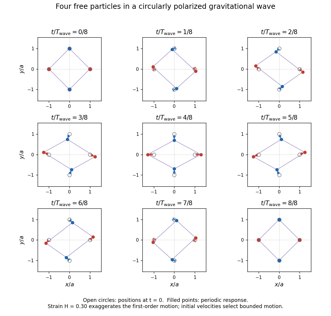
One full circularly polarized gravitational-wave cycle, with the four particles at their specified initial positions at phase zero
. Details. 
Gravitational radiation admits polarization: general relativity has two transverse tensor modes, plus polarization and cross polarization, whose relative amplitudes and phase give linear, elliptical or circular gravitational-wave polarization. Their axes transform through twice a rotation of the transverse coordinate frame, unlike the vector polarization of electromagnetic radiation. Measuring these modes is physically plausible with several differently oriented detectors; a single detector generally measures only one projected combination.
Gravitational waves can exhibit interference. In linearized gravity, overlapping strains add, so coherent contributions can enhance or cancel the measured response. Independent astrophysical sources generally have unrelated phases and average to a stochastic background rather than stable fringes. More plausible coherent paths arise when gravitational lensing sends different parts of the same signal to the detector with different delays; fringes require sufficient overlap and coherence. The relevant quadratic radiative energy flux contains the cross terms even though the leading wave equation is linear.
In a local inertial frame in vacuum, gravitational waves travel at in general relativity; there is no ordinary material index of refraction analogous to a transparent dielectric. Ordinary matter couples so weakly that laboratory prisms for gravitational waves are implausible. Propagation through a varying background gravitational field nevertheless changes ray directions and travel times, giving gravitational lensing and Shapiro time delay. In weak static coordinates , the null condition gives an effective coordinate index of refraction . This useful description depends on coordinates and does not change the local propagation speed. Thus astronomical gravitational refraction is plausible, while a substantial everyday material effect is not.
Gravitational waves also exhibit diffraction: the geometrical optics ray description fails when a propagation structure or lens delay is not large compared with the wave's wavelength or period. For a compact lens of mass , a useful dimensionless parameter is ; of order one signals potentially appreciable wave effects, with cosmological lens redshift supplying an additional factor when needed. Astrophysical gravitational lensing can therefore produce diffraction and frequency-dependent amplification. Ordinary objects are poor opaque screens for gravitational waves, so everyday slit-and-screen demonstrations are implausible despite the large wavelengths, which are about km at Hz.
The intended orbit is a freely falling timelike circular Schwarzschild geodesic. Use the Schwarzschild metric with rather than as the zeroth coordinate, and put the orbit at . Thus , , , with . The radial geodesic equation at constant isConsequently . The four-velocity normalization givesand henceHere is Schwarzschild time, the orbiting clock's proper time, the gravitational constant, the central mass, the constant areal radius, and the speed of light. The dimensionless follows the question's time-valued zeroth-coordinate convention; with the zeroth four-velocity component would be .
The condition is for a massive circular geodesic; radial stability further requires , with equality marginal. The phrase “any circular orbit” is false without free fall: a powered circular trajectory has with independently chosen . For example, at choose ; this valid accelerated circular trajectory has , instead of the displayed .
Let , , , and choose . A torque-free test gyroscope moving on a geodesic has a spin four-vector obeying parallel transport,The orthogonality condition says the temporal spin component vanishes in the body's rest frame, not necessarily in Schwarzschild coordinates. Here it givesIn addition to the radial Christoffel symbols in part (a), use and . On the equator the parallel transport equations becomeThe radial equation follows by substituting into . Eliminating gives .
Let be the invariant spin magnitude. Initially radial spin means and . The complete solution isTo interpret the orientation, convert coordinate components into the orbiting orthonormal frame. The Lorentz factor relative to a Schwarzschild static observer is , so the body's measured radial and tangential spin components areTheir squared sum is , and their angle relative to the outward radial direction decreases uniformly at rateThe differing coordinate amplitudes in must not be interpreted as a nonuniform physical spin rotation. After one orbital period the radial basis has turned by while the spin has turned by relative to it. The residual geodetic precession is in the orbital direction.
For a timelike circular Schwarzschild geodesic, the coordinate orbital period and onboard proper time per orbit areUsing and , the Schwarzschild radius and orbital areal radius are and . ThereforeThe crew accumulates about fewer seconds, or fewer minutes, per orbit. Both gravitational time dilation and kinematic time dilation contribute: a static clock at has , while the orbiting clock additionally has , where . A distant observer measures the coordinate period; comparing arrivals emitted at the same orbital phase also removes the repeated light propagation delay.
The geodetic precession per orbit isThe orbital position and four-velocity repeat after a full orbit, so the direction to distant Earth in the instantaneous rest frame repeats. The freely transported gyroscope does not: its beam axis has turned through relative to the original aiming direction. This applies to any initial in-plane spin direction by linearity of parallel transport, not only the radial initial condition used in part (b). The beam's angular diameter is , giving a half-angle of . Thus Earth lies outside the beam after one orbit; comparing the offset with the diameter would already show a miss, but the correct acceptance angle is the half-angle.
The initial radial ray must be outward from the black hole for a direct path to Earth. A precisely inward radial null geodesic falls into the black hole and cannot provide the assumed initial communication. For outgoing near-radial Schwarzschild light deflection, the angular correction is especially small. If a static observer at measures a small emission angle from the outward radial direction, its impact parameter is . The outgoing null geodesic givesRelative to flat propagation, curvature changes the small pointing angle and beam radius by the fraction . At an offset of this is only about ; the beam's radius changes by about . The exactly radial central ray has zero angular deflection. This is not the geometry of the usual scattering formula, which assumes a ray coming from infinity, passing the black hole, and returning to infinity.
Relativistic aberration also distinguishes a coordinate-radial light ray from a beam aimed radially in the moving crew's frame. Here . Successful initial aiming includes that fixed correction; the same correction applies at the repeated orbital position. More precisely, an outgoing static-radial ray initially has crew-frame angle from the radial axis. The local small-angle aberration factor about that aim is ; including the outgoing propagation factor gives . Thus the asymptotic miss is about and the beam half-angle about , with the same conclusion. The small distortion of the outward beam cannot correct the much larger accumulated geodetic precession.
On large scales the appropriate background is the spatially flat FLRW metric,Here is cosmic time, the proper time of a comoving observer; is the scale factor; and are dimensionless comoving coordinates. With this convention has units of length. A fixed comoving radial interval has instantaneous proper length . The cosmological principle assumes spatial homogeneity and cosmological isotropy on the scales where this background description applies.
The general FLRW metric instead has in its radial part, with normalized describing positive, zero or negative spatial curvature of an FLRW universe. The best simple description takes ; observations constrain spatial curvature to be small rather than proving it identically zero. The late accelerated expansion is encoded by the time dependence of , determined by the stress-energy tensor through the Friedmann equations, rather than by an additional term in the FLRW metric. Small-scale galaxies and other inhomogeneities require perturbations of this background.
For a perfect fluid in general relativity, let be rest-frame total energy density divided by , its isotropic pressure, and its four-velocity, normalized by . ThenThe contracted Bianchi identity and the Einstein field equations give stress-energy conservation, , for a constant cosmological constant. Contract with and use the normalization to obtainIn comoving coordinates and the covariant divergence is , where a dot is a cosmic time derivative and the Hubble parameter. ThereforeFor a fixed region in comoving coordinates, let be its physical volume, where is a fixed coordinate-volume integral, and let . Since ,Thus the cosmological perfect-fluid continuity equation is exactly equivalent to the adiabatic first law of thermodynamics, , for every nonzero such region. Conversely, expanding that first law of thermodynamics and dividing by recovers the same equation. No heat or particle flux crosses the comoving boundary; interacting components separately need source terms, although the total still obeys this conservation equation.
There is a sign inconsistency in the supplied formula sheet worth isolating. Its Riemann curvature tensor and Ricci tensor conventions, together with its stated metric signature, give for with constant . Its vacuum Einstein field equations with then require , whereas its printed vacuum Friedmann equation gives . For example, , and satisfy the latter but leave the former's component equal to . Changing the geometric cosmological constant term to repairs this mismatch. The conservation derivation is unaffected; below take the geometric cosmological constant to be zero and include any vacuum energy as a fluid, so no ambiguous sign enters.
Write the equation of state as . Integrating the cosmological perfect-fluid continuity equation for constant gives . With spatial flatness and the geometric cosmological constant set to zero, the Friedmann equation is .
In S1, describes vacuum energy: and is constant. Its negative pressure drives accelerated expansion, , and the expanding solution is . This is the ideal de Sitter spacetime approximation to cosmic inflation. An exactly constant vacuum component cannot end its phase unaided; a phase transition or reheating mechanism is required for the assumed change to S2.
In S2, describes an isotropic bath of ultrarelativistic particles, such as photons, with negligible rest mass relative to their energy. The number per physical volume falls as , while the energy per particle redshifts as , so . This radiation-dominated universe has on its expanding branch.
In S3, describes pressureless matter, or relativistic dust, with negligible random kinetic energy. Conserved particle number and approximately fixed rest energy give . A flat universe containing only this component is the Einstein-de Sitter universe, with . The constants are integration offsets in the individual phases; they need not represent one common start time when phases are matched.
For monotonically expanding scale factor , , so the elapsed cosmic time isThe second expression uses cosmological redshift ; the age of the universe is the limit to its earliest specified state, if that limit is finite.
An age comparison for an initial vacuum-dominated phase needs a common normalization. Match the two histories at the end of S1, with and , and give them identical subsequent S2 and S3 evolution, including transition radii and today's state. Below , the history with S1 has constant . The comparison history extends S2 backwards, so and . Starting both at , where , their early durations areThe difference is positive becauseThe common later evolution adds the same time to both histories. Thus S1 makes this matched universe older. More strongly, as , the exact S1 duration diverges logarithmically, whereas a radiation beginning has finite duration to the match. The exact de Sitter spacetime expanding patch reaches only as for its comoving observers; a finite “age since ” does not exist in this ideal model. This does not establish past geodesic completeness of the patch.
The matching assumption is essential for a finite cutoff or realistic finite period of cosmic inflation: arbitrary changes of the present Hubble parameter or transition densities prevent a universal age comparison. The literal zero-size limit in this question is instead the infinite-duration idealization just derived.
The actual large-scale expansion is well described by the Lambda-CDM model: radiation in cosmology, ordinary baryonic matter, cold dark matter and late-time dark energy coexist. A component becomes dominant through continuous changes in their density ratios, rather than every previous component disappearing at an instantaneous phase boundary. Matter pressure is small in its nonrelativistic regime, but radiation persists, and massive neutrinos interpolate between relativistic and nonrelativistic behavior.
There is also a late accelerated era, absent from a model ending permanently in S3. It is consistent with nearly constant vacuum energy, whose negative pressure eventually dominates because pressureless matter dilutes as . The scale factor then ceases to follow the pure Einstein-de Sitter universe law.
An early phase of cosmic inflation is a well-motivated model rather than a directly observed exact phase. Successful cosmic inflation must end and transfer its energy to matter and radiation through reheating; realistic models generally have slowly varying and close to, rather than exactly equal to, . Extrapolating a strictly constant to arbitrarily small is not a measurement of the universe's past duration. Finally, spatial homogeneity and cosmological isotropy apply statistically on large scales: galaxies, gravitational waves and other perturbations are absent from the exact FLRW metric, and small spatial curvature remains an observational possibility.
Articles by others on the same topic
There are currently no matching articles.