Past exam of the mathematics course of the University of Cambridge / 2001 / iii / Paper 47 (Mechanics of Elastic Solids)

Let $B=A^{\mathsf{T}}A$. Since $\det A>0$, $B$ is a positive-definite matrix. The spectral theorem gives a unique principal square root of a positive semidefinite matrixThen $R^{\mathsf{T}}R=U^{-1}B{U}^{-1}=I$ and $\det R=\det A/\det U=1$, so $R$ is a rotation matrix. Define $V=RU{R}^{\mathsf{T}}$. It is a symmetric matrix, is positive definite, and satisfies $V^2=A{A}^{\mathsf{T}}$. Consequently the polar decomposition in continuum mechanics isHere $U$ and $V$ are the right stretch tensor and left stretch tensor.

For the Cauchy stress tensor, use both material isotropy and material frame indifference. Their respective transformation laws areThe first law and $A=VR$ give $\sigma (A)=\sigma (V)$. Combining the two laws gives $\sigma (QV{Q}^{\mathsf{T}})=Q\sigma (V)Q^{\mathsf{T}}$. In a principal stretch basis, $V=\mathrm{diag}({\lambda }_1,{\lambda }_2,{\lambda }_3)$. Each half-turn about a coordinate axis leaves $V$ unchanged; its conjugation changes the signs of the corresponding off-diagonal stress tensor entries. Those entries must therefore vanish. If two principal stretches coincide, rotations within their eigenspace additionally force the stress tensor to be scalar on that eigenspace. Thus the Cauchy stress tensor and left stretch tensor have common principal axes, including at repeated principal stretches. This proves coaxiality of isotropic elastic stress.

The precise symmetry conclusion is equivariance of isotropic principal stresses. Every permutation of the principal stretches can be realized by a signed permutation rotation matrix, sowhen the indexing is permuted consistently. Equivalently, permuting the arguments permutes the labelled principal stresses in the same way. In particular, ${\sigma }_1$ is symmetric in ${\lambda }_2,{\lambda }_3$, and analogous statements hold for ${\sigma }_2,{\sigma }_3$.

For distinct principal stretches, interpolate the three values ${\sigma }_i$ at the three points ${\lambda }_i$:Uniqueness of this interpolation implies that the scalar coefficients ${\beta }_j$ are symmetric functions of the unordered principal stretches; they may be expressed through the elementary symmetric invariants. Smooth isotropic constitutive laws have the corresponding invariant representation across repeated stretches as well. The wording about symmetric functions must be understood in this collective sense: each labelled principal stress need not be symmetric in all three arguments. For example, the objective isotropic law $\sigma =V^2$ has ${\sigma }_i={\lambda }_i^2$, which disproves that stronger interpretation.

Use material coordinates $X$ and write the placement as $y=X+u$. The strain energy density $W$ in the printed convention is per unit reference mass. It is convenient to use the conventional first Piola-Kirchhoff stress tensor $P=s^{\mathsf{T}}$, soAssume the undeformed reference state is stress-free. With $H=A-I$ and infinitesimal strain tensor $e=(H+H^{\mathsf{T}})/2$, material isotropy and material frame indifference give the quadratic expansionConsequently the Lamé parameters from hyperelastic energy Hessian areIndeed, differentiating the quadratic expression twice givesthe elastic stiffness tensor of linear elasticity. A prestressed reference state requires the corresponding initial-stress corrections; the displayed formula concerns the natural state.

For a plane elastic wave, $u=u(X_1,t)$, put $r=e_1+u_{,X_1}$ and $\Psi (r)=W([r,e_2,e_3])$. Balance of momentum without body force becomesThis is a material-coordinate equation: the reference density cancels between inertia and nominal stress. If $C{a}_{\alpha }=c_{\alpha }^2{a}_{\alpha }$, the first-order system has characteristic speeds $\pm c_{\alpha }$ and right eigenvectors $(a_{\alpha },\mp c_{\alpha }{a}_{\alpha })$. Along a characteristic curve with $d{X}_1/dt=s=\pm c_{\alpha }$, its differential compatibility relation isThis follows by multiplying the system by the left eigenvector $(-s{a}_{\alpha }^{\mathsf{T}},a_{\alpha }^{\mathsf{T}})$. It does not assert the existence of globally integrable Riemann invariants for an arbitrary three-component constitutive law.

There is a necessary qualification to the finite-amplitude transverse request. Set $u=(0,w,0)$ and $q=w_{,X_1}$, so $r=(1,q,0)$. The longitudinal momentum equation requiresThus arbitrary nonuniform pure transverse profiles are possible only if the compatibility condition for pure nonlinear transverse waves holds:The third component vanishes by the reflection symmetry implied by isotropy and objectivity. The shear equation then closes:

General compressible hyperelastic material assumptions alone do not imply the required compatibility. For a concrete counterexample, take the Saint Venant–Kirchhoff hyperelastic energyFor $A=[(a,q,0{)}^{\mathsf{T}},e_2,e_3]$, this becomesAt $a=1$, $P_{11}=(\lambda +2\mu )q^2/2$. A varying shear therefore produces a longitudinal force $(\lambda +2\mu )q{q}_{,X_1}$ and cannot preserve $u_1=0$. Infinitesimal transverse waves do exist, because this coupling is second order, but a general pure finite-amplitude transverse wave does not.

The compatible nonlinear shear energy class is nonempty and can be genuinely nonlinear. Define $J=\det A$, $S=\mathrm{tr}(A^{\mathsf{T}}A)-2J$, and, for $h\ge 0$, takeThis is objective and isotropic. Near $A=I$, $S-1=2\mathrm{tr}(e^2)-(\mathrm{tr}e{)}^2+O(|H{|}^3)$, so it has the specified Lamé parameters. On the plane deformation above, $S-1=(a-1{)}^2+q^2$ and $J=a$. Hence $P_{11}=0$ at $a=1$, whileFor positive $\lambda ,\mu$, the relevant incremental plane moduli are positive. This supplies an explicit stable pure transverse family and, when $h>0$, amplitude-dependent wave speed.

For any compatible family, letThe equations $q_t=v_{,X_1}$ and $v_t=c(q{)}^2{q}_{,X_1}$ give the Riemann invariantsConsider the initially undisturbed half-space $X_1>0$. A right-going simple wave has the incoming invariant $v+H=0$, so $v=-H(q)$. Denote the prescribed boundary nominal stress by $T(t)=P_{21}(0,t)=\tau (q_b(t))$. The physical boundary traction, whose outward normal is $-e_1$, is $-T(t)e_2$. Invert the monotone law $\tau$ to obtain $q_b$. The wave state emitted at boundary time $s$ is transported alongAhead of the leading front $X_1=c(0)t$ the state is zero. Before characteristic crossing, these equations determine the unique emission time $s$ for each disturbed point. The displacement itself is also determined, rather than just its derivatives:Differentiating the implicit emission relation verifies $w_{,X_1}=q_b(s)$ and $w_t=-H(q_b(s))$, so this is the complete pre-shock simple wave solution.

Write $c_b(s)=c(q_b(s))$. The boundary-generated characteristic curves lose invertibility whenThus the characteristic crossing in a boundary-generated elastic simple wave criterion isHere ${\dot{c}}_b=c^{\prime }(q_b)T^{\prime }/({\rho }_0{c}_b^2)$. A smoothly increasing boundary stress therefore steepens into a shock wave only when later states travel faster: $c^{\prime }(q_b)T^{\prime }>0$. Increasing stress alone is insufficient. For the compatible example with $h>0$ and $q_b>0$, $c^{\prime }(q_b)=3h{q}_b/({\rho }_0{c}_b)>0$, so a nonzero increasing ramp produces finite-time crossing. For $h=0$ all rays are parallel and no such shock forms. This criterion locates the first gradient singularity; subsequent discontinuous evolution additionally requires the jump conditions and an admissibility condition.

For a general vector simple wave, replace the pure-shear line by an integral curveSubstitution gives $a_t+c_{\alpha }(a)a_{,X_1}=0$, with the same emission construction and crossing criterion. Boundary tractions must lie on this one-family curve. Generic finite-amplitude quasi-transverse waves may contain longitudinal displacement; arbitrary vector boundary forcing need not generate a single simple wave.

Take the difference $w$ of two solutions with the same body force, initial displacement and initial velocity. It satisfies the homogeneous linear elasticity equations. With $e=e(w)$ the infinitesimal strain tensor, define the bulk energyThe usual stability assumptions make the elastic quadratic form nonnegative and $\rho >0$. Multiplying momentum balance by $w_t$, using integration by parts and using symmetry of the stress tensor givesAll interior terms cancel: the strain term is exactly the time derivative of elastic energy.

For the restoring boundary law, $t_w=kw$. The prescribed support displacement cancels in the difference. Since $k$ is a time-independent symmetric matrix,Hence the elastic energy uniqueness with restoring boundary springs identity isThe boundary contribution is nonnegative because $k$ is negative semidefinite. The initial difference and its velocity vanish, so the conserved energy is zero. Its kinetic term implies $w_t=0$ everywhere; the zero initial displacement then gives $w=0$. This proves uniqueness without needing to exclude rigid displacements separately.

Physically, $-k$ is a nonnegative boundary spring-stiffness matrix, and the prescribed vector $U$ is the moving support position. The traction restores the displacement towards that support; null directions of $k$ have no spring force. The interpretation and conserved-energy proof use a fixed spring matrix, as indicated by the given boundary law.

On the mixed part $S_1$, write $t=\sigma n$. The condition isThus the tangential traction and normal displacement are prescribed. The normal traction is a constraint reaction; tangential displacement is free. Only the tangential component of $F$ matters. On $S_2$, the entire displacement is prescribed.

For the difference of two such solutions, $w\cdot n=0$ and $(I-n{n}^{\mathsf{T}})t_w=0$ on $S_1$. Consequently $w_t$ is tangential and $t_w$ normal, so $w_t\cdot t_w=0$. On $S_2$, $w_t=0$. The boundary power vanishes everywhere, giving $d{E}_{\mathrm{bulk}}/dt=0$. The same zero-initial-energy argument gives $w=0$. Therefore the mixed boundary problem also has at most one solution.

Use the local momentum equation in the current volume:Symmetry of the Cauchy stress tensor and the product rule giveApply the divergence theorem and use $t_j={\sigma }_{jk}{n}_k$. The mean stress and strain boundary identities follow:For infinitesimal strain tensor, $e_{ij}=(u_{i,j}+u_{j,i})/2$, and a second application of the divergence theorem gives

To first order, evaluate self-gravity in the undeformed uniform sphere. The shell theorem says that only the enclosed mass $M(r)=4\pi \rho r^3/3$ contributes to the inward field. ConsequentlyThe field vanishes at the centre and increases linearly to its surface value.

The requested radius change concerns the final traction-free static elastic equilibrium, not the acceleration immediately after gravity is switched on. In equilibrium the boundary traction and acceleration vanish. Spherical symmetry givesThe homogeneous linear elasticity law commutes with volume averaging:Thus $\overline{e}=e_{0}I$ with $e_0=-\rho ga/(15\kappa )$. This conclusion is about the mean strain, not a claim that the local strain is uniform.

Let the boundary displacement be $u(a)=u_{a}n$. Since ${\int }_S{n}_i{n}_{j}dS=(4\pi a^2/3){\delta }_{ij}$, the boundary identity gives $\overline{e}=(u_a/a)I$. Therefore the equilibrium contraction of a self-gravitating elastic sphere isThe shear modulus cancels because the mean deformation is purely volumetric.

The full radial field provides a useful check without assuming uniform deformation. For $u=f(r)e_r$, momentum balance isRegularity at the centre gives $f=Ar+B{r}^3$, withfrom ${\sigma }_{rr}(a)=0$. Substitution reproduces $f(a)=-\rho g{a}^2/(15\kappa )$. During the transient, the acceleration term in the mean-stress identity remains; gravitational feedback from the small density and shape changes is higher order in the equilibrium calculation.

Write $n=(x-\xi )/R$ for the receiver direction. With the printed time convention $e^{i\omega t}$, an outgoing spherical wave has phase $e^{-i\omega R/v}$. The leading terms of the elastodynamic Green tensor are of order $1/({\alpha }^{2}R)$ and $1/({\beta }^{2}R)$, while the remaining terms have orders $1/(\omega v{R}^2)$ and $1/({\omega }^2{R}^3)$. Thus the far-field approximation requiresThis is an absolute asymptotic comparison of the tensor terms. At an angular node of a leading radiation component, the smaller near field can still dominate that component. The PDF prints an opposite phase sign in the near-field shear exponential; that would be incoming with this time convention. The outgoing leading terms, which determine all the requested far-field patterns, are unambiguous.

For a unit time-harmonic point force in direction $d$, the far-field P and S radiation from a point force isThe normalization here follows the given elastodynamic Green tensor; a separate force-density convention would include its corresponding density factor. If $\theta$ is the angle between $n$ and $d$, the signed radial P wave amplitude is $\cos \theta$, and the magnitude of the S wave amplitude is $\sin \theta$. The P wave has two oppositely signed lobes and a nodal plane perpendicular to $d$. The S wave is polarized in the projection of $d$ onto the receiver's tangent plane, has nodes along $\pm d$, and has its maximum on the perpendicular great circle. Rotating its planar section about $d$ gives the full toroidal S wave magnitude pattern.

For a point source with seismic moment tensor $M$, convolution with the derivatives of the Dirac delta function gives $u_i=M_{jk}{\partial }_{{\xi }_k}{G}_i^j$. In the far field, differentiating the outgoing phase contributes $i\omega n_k/v$; differentiating $R^{-1}$ or $n$ is a lower-order effect. Thus the point-moment elastodynamic displacement is

The double couple has $M=e_1{e}_2^{\mathsf{T}}+e_2{e}_1^{\mathsf{T}}$. Its double-couple radiation pattern therefore has signed radial P wave factor and tangential S wave vectorIn the $x_1{x}_2$ plane, $n=(\cos \varphi ,\sin \varphi ,0)$, giving $A_P=\sin 2\varphi$ and $A_S=\cos 2\varphi$, where the signed S wave component is along $(-\sin \varphi ,\cos \varphi ,0)$. The P wave nodal planes are $n_1=0$ and $n_2=0$, and the alternating lobes peak on their bisectors. The planar S wave lobes peak along the coordinate axes. For the complete three-dimensional pattern, write $n=(\sin \theta \cos \varphi ,\sin \theta \sin \varphi ,\cos \theta )$:The full S wave has additional zeros at $\pm e_3$ as well as at the planar bisectors.

For the explosion source, $M=I$. Then $n^{\mathsf{T}}Mn=1$ and $(I-n{n}^{\mathsf{T}})Mn=0$. The explosion radiation in an isotropic elastic solid is therefore an isotropic radial P wave, with no S wave radiation. A dilatational point source is a gradient source; its far-field force is parallel to the propagation direction, so the transverse projection vanishes.

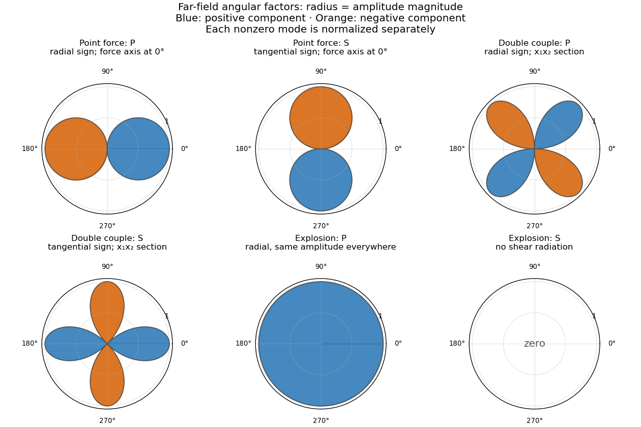
Each radius in the sketch is the magnitude of the angular factor, separately normalized for each mode. Blue and orange distinguish signs of the indicated radial or tangential component. The point-force sections contain its axis; the double-couple sections are in the $x_1{x}_2$ plane. The formulas above specify the full three-dimensional patterns.

Use the usual minor and major symmetries of the elastic stiffness tensor, positive density, and strong ellipticity in elasticity. For the plane elastic wave $u=a{e}^{ik(n\cdot x-vt)}$, substitution into momentum balance gives the acoustic tensor problemThe major symmetry makes $\Gamma$ a real symmetric matrix. Moreover $a^{\mathsf{T}}\Gamma a=c_{ijpq}{a}_i{n}_j{a}_p{n}_q>0$ for nonzero $a$ under strong ellipticity in elasticity. Hence its three eigenvalues are positive and the three positive wave speeds are real. Symmetry alone proves only reality of $v^2$: an unstable isotropic tensor with negative shear modulus has negative transverse $v^2$. The requested reality therefore uses stability as part of the physical elastic-solid assumption.

The elastic slowness surface consists of three sheets, with $s=n/v_{\alpha }(n)$, satisfyingIt is centrosymmetric. Sheets can meet at degenerate polarizations; they need not be spherical or convex in an anisotropic solid. The group velocity is normal to the corresponding smooth sheet: for a sheet tangent $ds$, differentiation of $a^{\mathsf{T}}[c_{ijpq}{s}_j{s}_q-\rho I]a=0$ gives $a_i{c}_{ijpq}{a}_p{s}_{q}d{s}_j=0$. The coefficient vector is proportional to the group velocity, so its scalar product with every tangent vanishes.

Fix horizontal slowness $p=(n_1/c,n_2/c)$ and put $q=s_3$. DefineThe symbol $p$ on a tensor index is an index, whereas $p_{\alpha }$ is a horizontal slowness component. The vertical slowness equation is the vertical slowness sextic of an anisotropic solidThe leading coefficient is $\det T>0$, so it is a degree-six polynomial with real coefficients. Nonreal roots occur in conjugate pairs, leaving between zero and six real roots counted with multiplicity. Generically the counts are $0,2,4,6$; a grazing repeated root can give an odd count of distinct real roots. Geometrically these are the intersections of a vertical line of fixed horizontal slowness with the three sheets.

All four generic counts are actually possible in a stable material. For example, take $\rho =1$ and orthotropic Voigt stiffnessesThe stiffness matrix is positive definite. For horizontal slowness $(p,0)$, the three diagonal acoustic equations areThe choices $p=0.1,0.3,0.8,1.2$ give respectively six, four, two and zero real vertical roots.

For the general depth-dependent amplitude, substitution of the horizontal harmonic factor yieldsFor six simple roots $q_{\ell }$, choose nonzero null vectors $a_{\ell }$ of the corresponding matrix. The complete solution isComplex vertical roots give evanescent waves. At defective repeated roots the usual polynomial-in-depth factors multiplying exponentials must be included, or the solution can be defined by a limiting procedure.

To classify the modes, take $x_3$ positive downwards and $\omega >0$. The reduced traction for a mode isMechanical energy crosses a plane at rate $-{\sigma }_{i3}{u}_{i,t}$. Averaging the real harmonic fields uses $⟨\mathrm{Re}(f{e}^{-i\omega t})\mathrm{Re}(g{e}^{-i\omega t})⟩=\mathrm{Re}(f{g}^{\ast })/2$. With velocity amplitude $-i\omega a_{\ell }$ and traction amplitude $i\omega b_{\ell }$, the time-averaged vertical acoustic energy flux isFor a real propagating mode, write its physical wavevector as $k=\omega (p_1,p_2,q)$. Differentiate $a^{\mathsf{T}}\Gamma (k)a=\rho \omega (k{)}^2{a}^{\mathsf{T}}a$ in $k_3$. The derivatives of $a$ cancel by the eigenvalue equation, while $a^{\mathsf{T}}({\partial }_{k_3}\Gamma )a=2\omega a^{\mathsf{T}}(Tq+R)a$. Thus its vertical group velocity and flux areThus the elastic mode classification by vertical energy flux is upgoing if $J_3<0$, downgoing if $J_3>0$. In anisotropy, the sign of vertical phase slowness alone need not classify energy propagation. For evanescent modes, select $\mathrm{Im}q>0$ for decay into a downward half-space and $\mathrm{Im}q<0$ for decay into an upward half-space. Away from grazing and degeneracy, continuation from zero horizontal slowness, with a small radiation damping if needed, separates three outgoing modes on each side. Superpose only the appropriate three to construct the most general upgoing or downgoing field; limiting modes handle exceptional cases.

For a free surface at $x_3=0$ with solid occupying $x_3>0$, let $(q_0,a_0)$ be a unit-amplitude incident upgoing mode. The reflected field consists of the three downgoing propagating or depth-decaying modes:Frequency and horizontal slowness are common to all modes, by translation invariance of the surface. Zero surface traction imposes the three equationsHence the free-surface anisotropic reflection amplitudes arewhenever $B$ is invertible. This specifies mode conversion as well as reflection. If $B$ is singular, a nonzero outgoing homogeneous surface mode exists; these are surface-wave poles, including Rayleigh waves in the isotropic case. At such parameters one must use the appropriate limiting radiation solution and check solvability instead of assuming a unique finite inverse.

Let the surface radius be $a$, let $\Delta$ denote epicentral angle in radians, and put $\eta (r)=r/v(r)$. The spherical elastic ray invariant gives $\sin i=p/\eta$. Along either radial leg, if $l$ is arclength and $\theta$ polar angle in the ray plane,For a turning ray with minimum radius $r_p$ defined by $\eta (r_p)=p$, the outgoing and incoming legs therefore giveThe square-root turning singularity is integrable for a regular turning point.

Introduce the reduced travel timeIts integrand vanishes at the moving lower endpoint, so differentiation gives ${\tau }^{\prime }(p)=-\Delta (p)$. Consequentlyon every regular travel-time branch. This is also the endpoint variation of travel time: the tangential endpoint slowness multiplied by the surface radius is $p$. Angles expressed in degrees would introduce the corresponding conversion factor; the displayed equality uses radians.

For Herglotz–Wiechert inversion, assume $\eta$ is strictly increasing so that $r=r(\eta )$ is single-valued, and set ${\eta }_a=a/v(a)$ and $h(\eta )=d\log r/d\eta$. The angular integral becomes an Abel integral equation:For any $0<\mu <{\eta }_a$, multiply by $(p^2-{\mu }^2{)}^{-1/2}$ and integrate. Interchanging the triangular region $\mu <p<\eta <{\eta }_a$ givesThe inner integral equals $\pi /2$: the substitution $p^2={\mu }^2+({\eta }^2-{\mu }^2){\sin }^2\theta$ reduces it to ${\int }_0^{\pi /2}d\theta$. Thus the full constructive inversion isThe surface radius and surface slowness fix the normalization. Varying $\mu$ reconstructs radius and speed parametrically; the centre is recovered by a limit when the data extend that far. The calculation assumes smooth regular turning rays and complete branch data, not merely the first arrival at each epicentral angle.

For a check, a constant speed $v_0$ gives ${\eta }_a=a/v_0$, $\Delta (p)=2\arccos (p/{\eta }_a)$ and $T(p)=2\sqrt{a^2-p^2{v}_0^2}/v_0$. These satisfy $dT/d\Delta =p$, and the inversion returns $r(\mu )=v_0\mu$.

If $\eta$ decreases outwards on an interval, then it increases as a surface ray travels inward through that interval. Such a ray cannot turn there, since turning requires the decreasing inward value of $\eta$ to reach $p$. Rays that penetrate this interval can traverse it and turn deeper, but the map $\eta \mapsto r$ now has several branches. The angular data constrain combinations of those branch contributions, rather than the single function $h(\eta )$ used above. This is a hidden turning-ray zone from nonmonotone spherical slowness. The stated single-valued inversion fails and does not uniquely locate the speed profile in that interval without additional information. Missing turning rays and possible multiple travel-time branches are the obstruction, not a failure of the algebraic Abel-kernel identity.