The cosmological principle asserts that, after averaging over sufficiently large scales, the universe is spatially homogeneous and isotropic on constant-cosmic time slices. Homogeneity means no distinguished location; isotropy means no distinguished spatial direction. These are statistical large-scale statements, not assertions that individual galaxies, clusters or the cosmic web are uniform, and they do not require the universe to be unchanging in time.
The nearly isotropic cosmic microwave background is strong evidence for large-scale isotropy about us. Its dominant dipole is explained by our peculiar velocity; the much smaller residual fluctuations provide the seeds and record of structure formation, rather than invalidating the principle. Large-area galaxy and radio-source distributions and deep galaxy surveys support statistical isotropy and a tendency towards statistical homogeneity after smoothing beyond the strongly clustered scales. An approximately isotropic Hubble flow and broadly uniform background radiation supply complementary checks.
There is an important logical distinction: isotropy seen by one observer alone does not prove homogeneity. A spherically symmetric inhomogeneous universe centered on that observer could look isotropic. Combining the observations with the assumption that our location is not privileged, so comparable observers would see comparable large-scale isotropy, motivates the homogeneous FLRW metric. Selection effects, foregrounds, finite survey volumes and the fact that observations lie on our past light cone must be accounted for. The evidence supports a large-scale statistical principle, not exact uniformity on every scale.
Use and signature . The positively curved FLRW metric in the usual radial chart isSet and introduce conformal time by . Then in the chart, and the spherical polar coordinate extends the spatial description to the full three-sphere. ThusThe coordinate itself is not one-to-one across the equator, which is why the new polar coordinate is useful.
For and , the Friedmann equation is . Since , it becomesFor pressureless matter, the background continuity equation gives . Define the conserved normalization . It makes the equation . The closed matter-dominated Friedmann solution is the cycloidIndeed and . Integrating gives the second expression, with the Big Bang at . It expands to at and recollapses at . Here is the constant appearing in the Friedmann equation; it is not the total mass of the entire closed spatial slice, whose volume is .
The luminosity distance is defined operationally by the bolometric relation for an isotropic source. It incorporates geometric spreading, reduced photon energy and dilated photon arrival times. If is the transverse comoving distance with the present scale factor included, then in a spacetime with an FLRW metric with photon number conserved.
Let be the emitted frequency. A narrow emitted band carries energy . At the observer the energy is smaller by , the time interval is , the frequency interval is , and the illuminated area is . Hence the spectral spectral flux density per unit observed frequency isFor the specified power law, , so the power-law spectral K correction isThere is no extra because is power per steradian. For total spectral luminosity , that factor would instead appear in the denominator. The frequency-band factor is essential: bolometric flux has two redshift-dimming factors, but spectral flux has one of them compensated by the bandwidth change.
Type Ia supernovae have similar peak luminosities that can be standardized using their light-curve width and color, rather than assumed to be identical without correction. Their redshifts and corrected apparent magnitudes give a distance modulus,Compare this Hubble diagram with the luminosity-distance prediction of a background cosmology. Restoring , put , and define as for , for , and for . ThenNeglecting radiation at these redshifts, Friedmann equations and a separately conserved dark energy component with giveFor constant , the last factor is ; a cosmological constant has . Thus the redshift dependence of the measured distance constrains matter density, curvature and the dark-energy equation of state. At small redshift, , showing how departures from the linear Hubble law probe the deceleration parameter.
The early distant-supernova analyses found larger distances than matter-only decelerating models predicted, providing evidence for accelerated expansion; see the 1998 supernova analysis and the 1999 independent supernova analysis. This is a statement about the distance-redshift curve under the standardization and cosmological assumptions, not a direct measurement of a fluid pressure.
The absolute magnitude–Hubble constant degeneracy means uncalibrated supernovae constrain the shape of without separately determining and the common absolute luminosity. The integral over also makes different matter, curvature and histories partly degenerate. Wide redshift coverage and independent cosmic microwave background and large-scale structure of the universe information help break these degeneracies. Dust extinction, source evolution, photometric calibration, sample selection and K corrections must be modeled, and constraints on a time-dependent equation of state depend on how that function is parameterized. Standardized supernovae test the expansion history; they do not by themselves uniquely determine every cosmological parameter.
Let be the density contrast, let be a comoving coordinate, and use . Define , so for the pressureless background. The perturbation Poisson equation isFor the comoving velocity field , local mass conservation givesOne obtains this by subtracting from . In the linear regime it reduces to , the linearized cosmological continuity equation. The spatial derivatives are with respect to , and the time derivative in the conservative continuity equation is at fixed . In contrast the acceleration of an individual fluid element is a material derivative. The physical peculiar velocity is .
Use and , where the growing linear growth factor obeys . The Poisson relation in part (a) immediately becomesAlong a fluid trajectory,Substitute this into the pressureless equation of motion to obtainThe growth equation cancels the second coefficient. By the definition of the logarithmic growth rate, , while . ThereforeThis is the printed when interpreted along the particle. Dividing the Eulerian continuity equation by instead givesThe density derivative in this conservative equation must be Eulerian. If both derivatives were read as material derivatives, the density equation would double-count advection; its material form is . These distinctions make the growth-time form of cosmological dust equations valid beyond the first-order terms, up to the single-stream pressureless-fluid limit. The reparameterization assumes .
For the growing density mode, write . The new Poisson equation gives with no time dependence. With periodic zero-mean or fixed decaying boundary conditions, this determines a time-independent up to a spatially constant, dynamically irrelevant function. ThusIn the linear continuity equation, , so . For the pure longitudinal growing mode, this gives and hence a time-independent scaled velocity. Equivalently, neglect the quadratic advection term in the motion equation and put . It obeysThe second expression follows directly from : its logarithmic derivative with respect to is the negative coefficient in the first equation. Excluding the homogeneous decaying-velocity component, , yields the pure growing-mode scaled velocityThe same holds along a trajectory to first order, since is second order.
The pure growing-velocity assumption matters. A growing density alone does not exclude a divergence-free decaying velocity. For example, in an Einstein-de Sitter universe with , one may add . Its divergence is zero, it solves the homogeneous linear motion equation, and it changes neither nor , yet it is not constant. Thus the printed constant-velocity statement is correct for the intended pure scalar growing mode; without that condition the displayed field is a counterexample. This extra mode is removed by the usual irrotational, no-decaying-mode initial conditions.
The condition is that the velocity be the pure irrotational growing-mode velocity, with the homogeneous component in part (c) absent. It is enough to impose and exclude additional harmonic or transverse motions through the boundary conditions. The linear equation for then keeps that difference zero. A time-independent velocity also forces the same equality in the linear motion equation when its coefficient is nonzero.
At first order the gradient can be evaluated at the initial position: shifting its argument by the first-order displacement changes the velocity only at second order. Integrate from to , givingThe trajectory is straight in comoving position as a function of growth time. The physical trajectory need not be straight or have constant physical peculiar velocity. This linear displacement relation is the basis of the Zeldovich approximation.
For the Zeldovich approximation, form the Jacobian matrix of the Lagrangian map:Let be the eigenvalues of this potential Hessian matrix, with the convention that positive means compression. Before shell crossing, conservation of the mass in a Lagrangian volume givesIf and is distinct from the other eigenvalues, the first singularity occurs at . One principal length collapses while the other two remain nonzero. The resulting cosmological caustic is locally a sheet, conventionally a pancake, rather than a simultaneous spherical point collapse. Degenerate equal eigenvalues can instead give line- or pointlike special cases.
The predicted density divergence signals failure of the single-stream description. If the straight Lagrangian displacements are simply continued, particles cross the sheet and keep moving along their original displacement directions. They are not slowed and trapped by the evolved self-gravitating multistream structure. The streams therefore separate again, producing excessively broad pancakes at late times. In an N-body simulation, the changing gravitational field pulls crossing streams back, produces repeated crossings and binds matter into more compact structures. This is the limitation described by Zeldovich pancake thickness after shell crossing. The initial-displacement extrapolation is useful through the onset of collapse, but does not supply the self-consistent post-crossing gravitational dynamics or virialization. After crossing, the physical density would require summing inverse absolute Jacobians over all streams, not using one negative determinant as a density.
In an Einstein-de Sitter universe, a slightly overdense spherical region initially expands nearly with the Hubble flow, with its early physical radius proportional to . Its extra self-gravity gradually slows its expansion relative to the background. The radius reaches a maximum at spherical-collapse turnaround, where the coherent radial velocity is zero; it then contracts. The ideal pressureless top-hat would collapse to a point, but real collisionless matter undergoes crossing and relaxation into a bound system with random motions and virial equilibrium.
The bound-shell solution illustrates the stages:At , and ; the formal cold collapse occurs at , . For a uniform isolated sphere, let . At turnaround , whereas the final virial theorem gives . Conservation of energy gives , henceThe usual spherical-collapse prescription associates virialization with roughly the formal collapse epoch, not with a literal instantaneous halt of the cold shell. The sketch distinguishes the formal point collapse from the schematic settling at the virial radius:
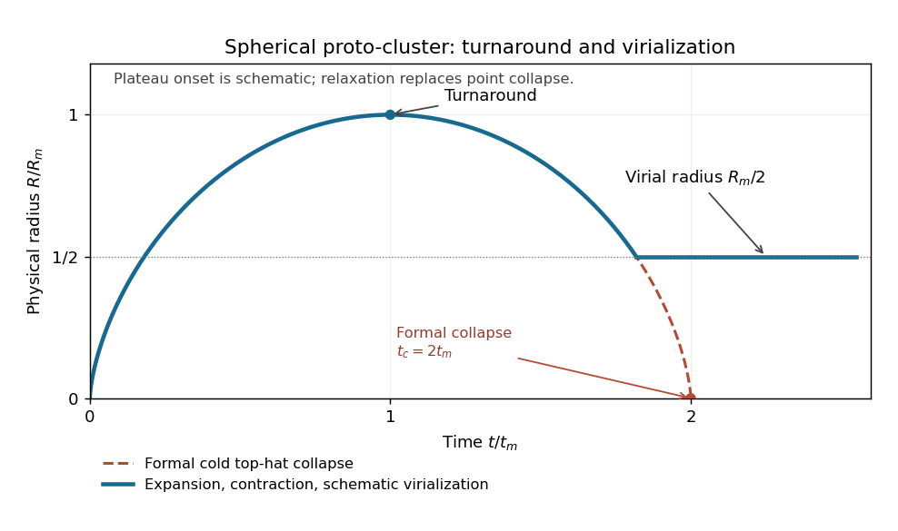
Spherical proto-cluster radius: expansion, turnaround, formal collapse and schematic virialization
. Details. 
The plateau onset is illustrative. A real cluster's relaxation, ongoing accretion and nonuniform density profile replace the cold solution, and surface pressure or energy exchange can change the half-radius estimate. The radius here is physical, not comoving.
For a uniform sphere of radius , write and . The self-gravitational potential energy is assembled by adding shells:The cosmological constant produces the external potential per unit mass , since in units . Its energy isThere is no additional factor for this fixed external potential, unlike the pair-counting factor for gravitational self-energy. At the maximum radius , the kinetic energy vanishes, soThis is the turnaround energy in uniform-sphere collapse with a cosmological constant. The original PDF's shell kinetic term is , not the produced by the TeX transcription.
For a homogeneous potential contribution of degree , the scalar virial theorem follows from the moment of inertia identity . Time averaging in equilibrium gives . Gravitational self-energy has degree , whereas has degree . Apply the theorem to the sum of the two contributions:With the uniform-sphere expressions this isThe cosmological-constant force is repulsive, so its virial contribution reduces the kinetic support required at a fixed radius. One must not apply the inverse-radius gravitational relation to the whole potential: the two terms have different homogeneity degrees.
Assume fixed mass, constant , no energy loss or surface work, and the same uniform-sphere structure coefficient at turnaround and virialization. Set and define the density in to be the mean turnaround density,It cannot be the background or final density if the displayed cubic is to hold with these coefficients. Put and . The turnaround energy is . At virialization, the relation in part (c) givesEquating the two energies and dividing by yields . Multiplication by givesThis derivation also fixes the density convention that the printed statement leaves implicit.
Differentiating the shell energy, or using its force, gives . At a genuine finite turnaround, and the acceleration must be inward. ThusEquivalently the turnaround radius is smaller than . The effective potential has its maximum at and second derivative . An initially expanding shell on the inner branch can turn around when its energy lies below this maximum; energy above it allows expansion over the barrier. The local inequality on is the turnaround bound with positive cosmological constant.
At the force vanishes at an unstable static radius. A shell approaching the maximum-energy separatrix reaches this radius only asymptotically, not at a finite expansion-to-collapse maximum. If it arrived there with zero velocity at finite time, uniqueness of the smooth radial equation would force it to have been the static solution already. Hence the inequality is strict for the turnaround used in the collapse calculation.
Use the physical root of the cubic which tends to as . For , the cubic has value at and value at , and its derivative is negative throughout that interval. Thus it has exactly one root there. Implicit differentiation givesThe smallest limiting value occurs as , since larger cannot have a finite turnaround. At the equation factors:The continuation of the collapsing root is thereforeThe lower endpoint is an infimum, not an attained minimum for a shell that turns around in finite time. This is the minimum virial-radius ratio with positive cosmological constant. The separate root at describes the limiting static situation and is not the collapse branch.
The smaller ratio does not mean vacuum repulsion makes turnaround easier. At fixed turnaround data, is more negative than for . If one tried , the virialized energy would be , which is not negative enough to equal . Extra contraction is necessary to increase the magnitude of the gravitational binding energy. Thus vacuum repulsion inhibits formation of a bound shell, while the shell that does form has a smaller idealized final-to-turnaround ratio under the stated energy and profile assumptions.
Optical cluster observations give galaxy positions and line-of-sight redshifts. Subtract the mean recession to obtain the line-of-sight velocity dispersion . If the tracers are in approximate virial equilibrium with isotropic velocities, and . Write the gravitational energy as , with determined by the density profile and radius convention. The virial theorem givesFor a uniform sphere , this becomes . Projected separations are commonly used to estimate a gravitational radius rather than literally assume a uniform sphere. Interlopers, substructure, anisotropy, tracer bias and a nonzero surface term affect the estimate. The inferred mass is total gravitating mass, not merely the galaxies' stellar mass.
For X-ray observations, the hot intracluster gas emits thermal bremsstrahlung and atomic lines. Spectroscopy determines its temperature, and the surface brightness, after deprojection, determines a gas-density profile. Under spherical hydrostatic equilibrium with thermal gas pressure, and . ConsequentlyThe order-of-magnitude virial version is . X-ray gas temperature is therefore a second measure of the depth of the gravitational potential. Nonthermal pressure, mergers, clumping and temperature gradients must be considered before equating the thermal estimate to the true mass.
For dense clusters the vacuum force is small compared with their internal gravity. If retained in the hydrostatic equation, it changes to and adds to the mass formula above. The optical virial relation likewise uses the separate vacuum contribution derived in part (c). Comparing optical and X-ray estimates tests the dynamical assumptions and exposes a gravitating mass much larger than the luminous stellar component.
Let be a mean-zero density contrast. For a statistically homogeneous and isotropic field, its two-point correlation function is , depending only on . For a galaxy point process the corresponding distinct-pair definition is , the excess pair probability relative to independent uniform positions. Self-pair shot noise is separated when using the density-field version.
Specify the Fourier convention byThe diagonal covariance follows from statistical homogeneity, and isotropy makes the matter power spectrum a function of alone. Substitute the inverse transforms into the correlation and integrate the delta function:Choose the polar axis parallel to . Angular integration gives . HenceConversely, when the transform is defined, . The stated convention fixes every factor.
Write . Using the transform in part (a), the band-limited linear density correlation isTwo integrations by parts give the antiderivative . Subtract its value at zero to obtain, for ,The origin is a removable limit. The bracket starts with , soThis is also the density variance obtained directly by setting in the integral. The sharp spectral edge produces oscillatory correlations, with leading large- term . A negative correlation at some separation is compatible with a nonnegative power spectrum.
Interpret the requested scale-dependent rms as the contribution from a logarithmic band of wavelengths, or equivalently a band centered at . A global uncut rms is not finite for this scale-free spectrum. The dimensionless density power per logarithmic wavenumber isThe cosmological Poisson equation gives . ThereforeThis is the potential fluctuations per logarithmic wavenumber scaling. A simple dimensional argument gives the same answer: the density amplitude on scale is proportional to , and its potential amplitude is of order , supplying two additional powers of .
For , the Harrison-Zeldovich spectrum has scale-independent potential amplitude per logarithmic interval. If the density-spectrum amplitude grows as , then , so the potential amplitude evolves as . It is constant in the pure growing matter mode of an Einstein-de Sitter universe, where .
A literal total variance would be proportional to . Infrared convergence requires and ultraviolet convergence requires , so no index makes both ends finite. At both divergences are logarithmic. Thus cutoffs or a band specification are essential for a numerical rms; the boxed statement describes the intended scale-local fluctuations rather than claiming a finite unsmoothed potential variance.
The Press-Schechter formalism starts from a statistically homogeneous Gaussian initial density contrast with variance specified by its linear matter power spectrum. Average it on mass scale , usually with a spherical top-hat. Let , normalizing consistently. Assume that a region becomes a collapsed halo when its linearly extrapolated smoothed density exceeds a mass-independent linear spherical-collapse threshold in the Einstein-de Sitter approximation. This extrapolates a linear Gaussian statistic to a nonlinear collapse criterion, and ignores the detailed nonspherical dynamics.
The one-scale Gaussian upper tail only assigns half the mass to overdense regions when the variance grows without limit. The conventional factor of two is inserted to account for material in larger collapsed regions even if it falls below the threshold on a smaller scale, the cloud-in-cloud issue. A first-crossing excursion-set argument can justify that factor for an ideal sharp-k filter; it is not a theorem that an arbitrary top-hat one-scale probability alone supplies it. With this prescription, the mass fraction in objects above isConvert mass fraction to comoving number density by assigning mass to each halo, using . This yields the Press-Schechter halo mass functionEquivalently one can use a present-extrapolated threshold and present variance; using both that threshold and an already grown variance would double-count growth. The model assumes approximate mass conservation, a smoothing-to-halo-mass assignment and a spherical universal barrier. It is an approximation to gravitational halo formation, not an exact partition of the real cosmic web.
In hierarchical formation, decreases with mass: smaller regions become nonlinear first and are subsequently incorporated into larger haloes. Define a characteristic mass by . It increases as growth proceeds, moving the exponential cutoff towards larger masses. For a scale-free spectrum with well-defined top-hat variance, , and hence . At a fixed mass, the derivative of with respect to is : rare high-mass abundances grow, while the small-mass abundance can decline as objects merge into larger systems. Thus one must not claim that every fixed-mass bin increases forever. The growth of is the scale-free characteristic mass in the Press-Schechter formalism.
For the temperature test, virial equilibrium and gas hydrostatic equilibrium give . Defining the halo radius by yieldsA calibrated monotone mass-temperature relation converts the mass function to , with temperature scatter treated by convolution when necessary. The cluster temperature function normalization is strongly sensitive to the linear fluctuation amplitude: at fixed mass and spectral shape, . Rare hot clusters occupy the exponential tail, so even a modest amplitude change can produce a large abundance change. Here sigma eight is the rms linear density contrast today in an top-hat, not the full spectrum.
Compare observed cluster-temperature counts and their redshift evolution with these predictions to constrain that normalization jointly with matter density and growth. The mass-temperature calibration, selection volume, temperature scatter, nonthermal support and deviations from the ideal halo mass function limit a temperature-only inference. The abundance of rare hot clusters is a sensitive amplitude probe once their mass calibration and cosmology are specified.
Articles by others on the same topic
There are currently no matching articles.