Use metric signature and initially set . For an internal scalar line with momentum , the Feynman propagator is . An -leg Feynman vertex, for , contributes , with all incident momenta incoming. Its in the Lagrangian density is canceled by the permutations of its identical fields. Each vertex conserves momentum and supplies . Integrate each independent loop momentum with , multiply the line and vertex factors, and divide by the Feynman-diagram symmetry factor for labeled external legs. Sum the distinct graphs and external-momentum assignments without counting the same assignment twice.
An unamputated momentum-space correlation function also contains the external propagators. Dividing the generating functional by its zero-source value removes disconnected vacuum bubbles; taking its logarithm selects connected correlation functions. Amputation of external propagators removes the external line factors when computing vertex amplitudes. Translational invariance leaves one overall momentum-conservation delta function for each connected graph.
The loop order is the number of independent graph cycles, equivalently the number of independent momentum integrations left after vertex conservation. A spanning tree through interaction vertices contains internal edges; hence, with internal lines,Restoring in gives for each internal propagator and for each interaction vertex. Thus an amputated connected amplitude hasThe same counting holds for a diagram in when the external source is coupled as : every external propagator brings , canceled by the source insertion's . This is Planck-constant loop counting with source normalization. An ordinary connected expectation of fields, with no such source factors, instead scales as ; multiplying by to form shifts its source-kernel counting to . The normalization must be specified when applying the printed loop rule.
Let count -valent interaction vertices. Counting their incident half-edges gives . Substituting the loop identity yieldsEach coefficient on the right lies between and , proving the vertex-count bounds for bounded scalar valenceThe free two-point term, which has no interaction vertex, separately satisfies the bounds with and .
A one-particle-irreducible Feynman diagram is connected and remains connected after any single internal line is cut. The left graph below contains two quartic vertices and two parallel internal lines: cutting either line leaves the vertices connected by the other. The right graph contains two cubic vertices joined by one internal line, whose removal disconnects it, so it is a one-particle-reducible Feynman diagram. Both have four external legs.
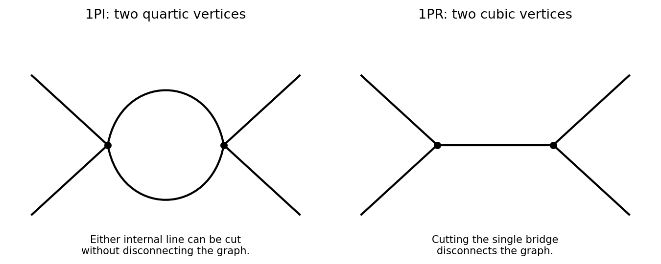
One-particle-irreducible quartic loop and one-particle-reducible cubic exchange with four external legs
. Details. 
The quantum effective action generates the one-particle-irreducible vertices. Their ultraviolet divergences and those of their proper divergent subgraphs are removed by local counterterms. Reducible connected graphs are reconstructed by joining these vertices with full propagators; they do not introduce independent local interaction counterterms merely because they contain bridges. This makes the one-particle-irreducible Feynman diagram decomposition useful for organizing renormalization. Overall power counting still has to be supplemented by subtraction of divergent subgraphs.
For a scalar with a two-derivative kinetic term, mass dimensions obeyThe general power-counting criterion used here is that interactions of nonnegative coupling dimension can be included in a perturbatively renormalizable quantum field theory, with all symmetry-allowed required local counterterms included; negative-dimensional couplings generally require an unbounded tower of higher-dimensional counterterms. Indeed, the scalar graph power-counting identity givesfor the superficial degree of divergence. Nonnegative coupling dimensions prevent this degree from increasing indefinitely with the vertex count.
The coupling dimensions areThus all three are power-counting renormalizable in three dimensions; cubic and quartic in four; cubic only in six. Positive-dimensional interactions are super-renormalizable, while the zero-dimensional ones are marginal by classical power counting. Usual kinetic, mass, vacuum and, when no symmetry forbids it, linear counterterms must also be admitted. This conclusion concerns perturbative ultraviolet renormalizability; it does not assert global stability of a cubic scalar potential.
Because is a real symmetric positive-definite matrix, its inverse exists and all its eigenvalues are positive. Completing the square givesThe translation has unit Jacobian determinant. Choose an orthogonal matrix with , where . The change also has absolute Jacobian one. The remaining integral is the product of one-dimensional Gaussian integrals, each equal to . Consequently the linear-source multivariate Gaussian integral isThe determinant square root is the positive one, as required by convergence of the original real integral.
A linear operator on finite-dimensional vectors acts by . For a field the discrete index becomes a continuous coordinate, and a suitable operator is represented by an integral kernel, possibly a distribution:The identity operator has kernel . If an inverse exists on the chosen domain and with the chosen boundary prescription, its kernel satisfieswith the analogous reversed identity. A differential operator is a distributional kernel: for example, . Its inverse is a Green function. Boundary conditions, a causal prescription and the treatment of zero modes are part of the inverse's definition, not consequences of formal matrix notation. An operator with an untreated zero mode does not have an inverse on the full field space.
The functional derivative is defined through the first variation: for arbitrary smooth test variation ,In particular,For a symmetric kernel, differentiating gives . The two terms from varying the two fields coincide; for a nonsymmetric kernel the symmetric part appears instead. Integration by parts is understood when is differential and the boundary variations vanish. A finite-volume, finite-mode regulator makes these statements ordinary matrix identities before a continuum limit.
Use the same metric signature as above and define the Minkowski generating functional byHere . Integration by parts writes the quadratic action as with ; the infinitesimal imaginary part damps the oscillatory Gaussian functional integral and selects the vacuum Feynman propagator. Abbreviating repeated spacetime integrations, completing the square givesTranslation of the regulated integration variables therefore yieldsThe source-independent normalization contains the regulated functional determinant and its oscillatory phase; it cancels in . Define . The Gaussian evaluation of a free scalar generating functional is equivalently .
With Fourier convention , acts as . The inverse-kernel equation then givesThis is the time-ordered free two-point correlation function: differentiating twice with respect to and multiplying by recovers . It obeys in the distributional limit. The is essential: the algebraic denominator alone would not distinguish Feynman, advanced and retarded Green functions.
For a finite-dimensional integral, . Expanding a polynomial interaction formally and interchanging each finite-order derivative with the regulated integral giveswhere is the free Gaussian integral. This is a perturbation-series identity; it does not assert convergence of the full expansion for an arbitrary potential.
For the Minkowski functional integral, each field insertion is generated byExpand , replace its field factors by these functional derivatives, and take the derivatives outside the free integral. The result is polynomial interactions as source differential operators:If the field interaction term contains derivatives of the field, the corresponding spacetime derivatives act on the source-insertion operators as well. For the scalar polynomial interactions the operator in the exponent isThe free quadratic source exponential then supplies all Wick contractions, reproducing the Feynman rules. For normalized correlation functions, divide the resulting interacting functional by ; the interaction operator changes this denominator too, so it cannot simply be ignored.
The renormalization-group beta function isAt one-loop accuracy, integrating givesFor a positive weak coupling and , the coupling increases toward the ultraviolet and decreases toward the infrared. Extrapolation predicts a Landau pole at , where the weak-coupling approximation fails. For , the positive coupling decreases toward zero as : this is asymptotic freedom. Toward the infrared it instead grows, so perturbation theory eventually fails. The zero coupling is a fixed point. If negative couplings are allowed mathematically, their direction of motion still satisfies , but the side on which the pole occurs reverses: for example approaches zero from below in the ultraviolet. Negative quartic coupling does not give a stable scalar potential.
For the loop calculation use , , and the PDF's vertex normalization . A Feynman parameter combines the denominators. Shift the Euclidean loop momentum to , and put . The regulated integral without the vertex prefactor isUsing Schwinger parameterization, , and the momentum Gaussian integral givesFor , , while the other factors have finite limits. Thus the massive scalar bubble pole in four dimensions isThis pole is independent of external momentum and mass and hence is canceled by a local quartic counterterm. There are three channels, corresponding to the three pairings of four external momenta. Their poles add, and a counterterm vertex cancels the sum whenThis is the total counterterm for the three four-point diagrams specified here. The minimal subtraction scheme removes their poles only. The one-loop tadpole is momentum independent and requires a mass counterterm, but does not produce one-loop wave-function renormalization; that is why it does not alter this one-loop coupling calculation.
The dimensionful bare coupling is thereforeIts independence of givesPutting , the finite coefficient of is . ThusThis is the one-loop quartic scalar beta function, positive for nonzero weak real coupling. The factors would look different with a regulator , but the four-dimensional beta function is unchanged. For massless theory take nonexceptional external momentum, or an infrared regulator, so an infrared singularity is not confused with the ultraviolet pole.
Absorb the gauge coupling into the connection and use . The anti-Hermitian generators make unitary for real parameters. With a matter field transforming as , require . Applying both sides to an arbitrary field givesExpanding and yields the infinitesimal gauge transformation with an anti-Hermitian connectionThe adjoint covariant derivative is . In components,The trace normalization makes the structure constants totally antisymmetric: and cyclicity of the trace supply antisymmetry in the remaining indices. Replacing by reverses the infinitesimal parameter convention and gives ; mixing the two conventions would change the ghost operator incorrectly. The trace normalization also gives the invariant quadratic form .
A gauge-invariant functional integral counts all representatives along each gauge orbit. The gauge condition selects a representative, and its delta functional enforces that selection. Assume a local patch where each orbit intersects the gauge slice once and the gauge-condition derivative has no residual zero modes. DefineChanging the orbit integration variable from to givesInsert this Faddeev-Popov gauge-orbit identity into the unfixed path integral. The action and measure are invariant under a change , so integration over factors out as the gauge-group volume. Dividing by that redundant volume leaves the fixed integral and its Faddeev-Popov determinant. In a perturbative patch with fixed determinant sign or phase, the absolute value is replaced by the oriented determinant, up to a field-independent normalization:Here . This is a functional determinant of the gauge-condition Jacobian, not an arbitrary extra weight. The local invertibility assumption matters: residual gauge transformations or multiple orbit intersections, described by the Gribov ambiguity, prevent treating this derivation as a global unique gauge slice without further qualifications.
Both extra factors can be incorporated into an enlarged action. An auxiliary real field Fourier-represents the delta functional, while a Grassmann Gaussian integral over independent Faddeev-Popov ghost fields represents the determinant:Thus the original fixed integral can be written with action and ordinary integration over the extra fields, with no explicit delta functional or determinant. The anticommuting fields give a determinant rather than the inverse determinant obtained from commuting Gaussian fields.
For the usual Gaussian family of gauges, add and integrate out . Completing the square producesThis is Gaussian gauge fixing with an auxiliary field; equivalently one averages the condition with its Gaussian weight. Gauge-invariant observables are unchanged apart from normalization. For the Lorenz gauge , the chosen transformation convention gives . The ghost action is , or after integration by parts. The dependence of on accounts for the ghost interactions.
Articles by others on the same topic
There are currently no matching articles.