Put . The planar autonomous differential equation isIts equilibria have , . There are none for , one at , and two for . At an equilibrium the stability matrix isWriting , is always a saddle equilibrium. At , the determinant is and the trace is : it is attracting for and repelling for .
At and , the eigenvalues are ; the nonzero quadratic term and parameter unfolding give a saddle-node bifurcation. At , the trace crosses zero at , with eigenvalues , giving a Hopf bifurcation. It is nondegenerate: around the equation is . At , a small oscillatory expansion of leading amplitude has , so the first nonlinear damping is positive and nonzero. For example, its second-order oscillatory expansion is with . Thus the small attracting limit cycle is on the side. At the matrix has a double zero eigenvalue and a nontrivial Jordan block, the Bogdanov–Takens bifurcation organizing the two curves. The local bifurcation curves areA change between node and focus away from these curves is not itself a local bifurcation.
For the requested global exclusion, suppose were periodic with period . Integrate the original equation over a period. The integrals of , , and vanish. ThereforeThe left side is nonnegative and the right side is negative when . This contradiction proves there are no periodic orbits for , independently of .
With the stated time rescaling, and , where primes refer to . Dividing by givesAt , put and define the HamiltonianIts orbital derivative is , so this is a conserved quantity. The Hamiltonian system has , .
For , set . The potential has a minimum at and a maximum at . The corresponding center equilibrium and saddle equilibrium have energies and . Levels contain closed ovals around , as well as separate unbounded components on the right. At , the center's ovals limit to a homoclinic orbit to the saddle, turning at . Its equation isThe same energy also has external unbounded saddle separatrices for . Levels above pass over the potential barrier and are open. Along the upper halves , so the closed loops are traversed clockwise. If , the two critical points coalesce into a degenerate equilibrium; if , the potential is strictly decreasing and there is no center or homoclinic loop.
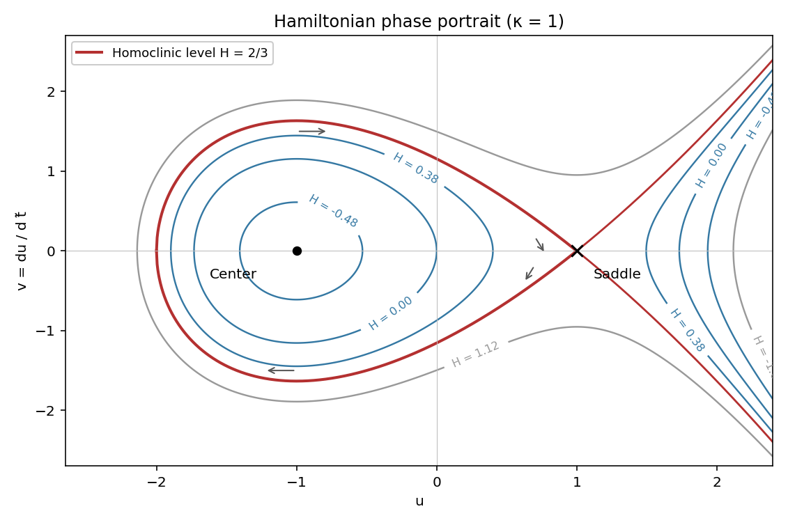
Hamiltonian level curves for kappa equal to one, showing the center, saddle and homoclinic loop
. Details. 
For small , the conserved quantity from part (b) instead obeys . The Melnikov energy-balance method evaluates the first-order net change along the unperturbed homoclinic orbit:Using the homoclinic curve , these are integrals of on its two halves. Their weighted mean is . Thus the first-order splitting vanishes at . Since its derivative with respect to is , the implicit function theorem gives a nearby curve where the stable and unstable saddle separatrices reconnect. This is the homoclinic balance for a quadratic-force oscillator and therefore a global, rather than local, bifurcation.
Returning to the original parameters, and . With fixed positive and , the homoclinic bifurcation curve has leading formThe energy integral locates the leading curve; the perturbed orbit itself is no longer a constant- curve.
With , the feedback system isFor , is an equilibrium. Its stability matrix and characteristic polynomial areThus there is always a zero eigenvalue, with eigenvector , so it is a nonhyperbolic equilibrium. If , the other two eigenvalues are off the imaginary axis: for their real parts are negative, while for their product is negative. At , all three eigenvalues are zero, explaining the exclusion in the next part.
Adjoin and use an extended centre manifold with local coordinates . Count as order , as appropriate to a steady-state fold, and writeThe centre-manifold invariance equation differentiates these graphs along . The derivatives and first contribute at weighted order three. Comparing the coefficients of and in the right sides therefore givesSince , their solution isHence the reduced normal form isBoth the quadratic and unfolding coefficients are nonzero, so the steady-state bifurcation is a saddle-node, with equilibria on the side. The exact steady equations confirm this: , , and , giving two nearby equilibria for and none for .
For the transverse modes are attracting; the negative- branch is locally attracting and the positive- branch has one unstable direction. For , one transverse eigenvalue is already positive, so neither full equilibrium is asymptotically stable, although the reduced fold is still present with reversed flow orientation. The parameter requires a higher-dimensional degeneracy analysis and is outside the stated assumption.
Assume a generic saddle-focus homoclinic orbit at , a smooth nondegenerate global reinjection along the selected unstable branch, and a sufficiently small neighborhood in which the linearized local flow supplies the leading passage map. Use linearizing coordinates if available; otherwise the calculation is a leading local approximation, not an exact consequence of eigenvalues alone. Choose the incoming section near in the plane , with coordinates where and . This section is transverse since . Choose an outgoing section . We mark one return after a global excursion; intermediate crossings of during the spiral are not counted as separate global returns.
In cylindrical coordinates the local flow isFor , the time to the outgoing section is . Set and . The outgoing coordinates areThe global part of the Poincaré return map is smooth around and takes the unstable-manifold point to . Expand it aswhere the coefficients may depend smoothly on and the matrix is generically nonsingular. Absorbing the fixed into them gives the leading two-dimensional return mapThe remainder refers to the smooth global-map Taylor approximation with bounded ; corrections to the local linear approximation are also neglected. The global map supplies the additive splitting parameter and the local map supplies the power and logarithmic rotation. For an iterated excursion on this same unstable branch, the next coordinate must again satisfy . A nonpositive image leaves this local return domain; the formula must not be iterated through negative logarithms.
For repeated small returns, , so is close to the nonzero constant . Retain its leading value in the second component. Combining into a single cosine, and absorbing the section size and fixed phases, gives the Shilnikov return mapChanging the sign of the logarithmic angle changes only the phase after using cosine's evenness. A generic reinjection has ; can be represented modulo by a positive value. The original PDF has exponent , which the converted TeX mistakenly replaced by .
This is an asymptotic scalar approximation, not an assertion that the full map has an exact one-dimensional invariant quotient. To see why it captures the thin geometry, differentiate the two components in part (a). Their determinant is of orderwhere involves and the determinant of the global linear map. For this tends to zero, so the return is strongly area-contracting even when its longitudinal derivative is large. Its global quadratic corrections are in this range. For a small fixed point, also , so ignoring contributes that same higher order. Multipassage iterates require all passage coordinates to stay in the small domain; the leading map describes their thin folded return geometry rather than controlling arbitrary points outside it.
Let . A fixed point of the Shilnikov return map is a periodic orbit with one marked global excursion, and satisfiesIts local passage takes logarithmically long. If the global travel time tends to , then its physical period isEliminating and absorbing section sizes and into constants and a phase gives the leading period–parameter relationFor the idealized leading map with a constant global travel time, the displayed two terms follow exactly; for the original flow, local and global approximation errors qualify their accuracy.
If , the oscillatory term is and . In a sufficiently small interval the map is a contraction. For there is a unique small attracting fixed point ; it is an attracting periodic orbit also in the transverse direction of the full return. For , for sufficiently small positive , so no periodic return orbit can remain wholly in this neighborhood. As from below, the attracting cycle becomes the homoclinic connection andContraction also excludes higher-period cycles wholly inside that small return neighborhood. This does not exclude remote periodic orbits elsewhere in the vector field.
If , the oscillatory term dominates . At the fixed-point equation isThere are infinitely many positive solutions approaching zero, with phases approaching successive zeros of cosine. Their leading ratio is , so their periods satisfy . At these roots the sine tends to , and the fixed-point multiplier has magnitude asymptotic to . Thus these are longitudinally unstable cycles, with the thin transverse direction contracting: infinitely many saddle periodic orbits accumulate on the homoclinic connection. Expanding oscillatory lobes produce interval-covering walks and horseshoe dynamics in suitable iterates; this is the positive-saddle-value case of the Shilnikov bifurcation.
Away from the connection, the one-passage branches wiggle in the period–parameter plane. To leading order,There is no single monotone logarithmic law: the phase matters, and the exponentially smaller term matters near cosine zeros. Folds occur when , asymptotically at . Their parameter values alternate in sign and accumulate geometrically toward zero. On a fixed-point branch, stability is ; small stable windows occur near stationary points of the oscillatory map. Crossing gives period-doubling bifurcations, while gives saddle-node bifurcations of periodic orbits. Subsequent doublings and chaotic invariant sets can occur; neither all periodic orbits being stable nor a particular universal sequence for every coefficient choice is implied.
For completeness, an -cycle of the return map, corresponding to a periodic orbit with global excursions, obeysand its total period isIts longitudinal multiplier is . This is the relevant period relation for multipassage cycles; substituting their total into the one-passage cosine law would generally be incorrect.
Use the group representation generated by the displayed matrices. The coordinate reflections generate , and the cyclic permutation conjugates to , then to . Thus the group is the semidirect product , of order . The converted TeX's multiplication sign must not be interpreted as a direct product of commuting factors.
To prove absolute irreducibility, complexify to and let be a nonzero complex invariant subspace. It is preserved by the coordinate projections . For a nonzero , at least one coordinate is nonzero, so is a nonzero multiple of a coordinate vector. Applying the cyclic permutation repeatedly shows that all three coordinate vectors belong to . Hence . Therefore the real representation is absolutely irreducible.
Equivalently, a commuting matrix must be diagonal because it commutes with all three reflections; commuting with forces its diagonal entries equal. This also confirms that every equivariant linearization is a scalar multiple of the identity, the condition needed in the branching calculation.
For the Equivariant branching lemma, assume a generic steady-state crossing after parameter normalization, and nonzero leading nonlinear coefficient on each axial line. The lemma gives an equilibrium branch for each axial subgroup with a one-dimensional real fixed-point subspace of a group action.
For , . Conjugation by supplies the other two coordinate axes. For , . Sign reflections supply all the equal-magnitude diagonals. These isotropy types are not conjugate: their subgroup orders are and . Thus there are two distinct primary axial branch types: coordinate-axis states and equal-magnitude diagonal states.
The global sign reversal belongs to the group and makes the restricted scalar equations odd, so generically each has the form , with . Its two nonzero solutions satisfy on the appropriate parameter side. Symmetry-related solutions belong to the same branch type; their existence does not imply stability or that both types lie on the same side of the crossing.
Equivariance under makes the first component odd in ; equivariance under and makes it even in . Up to cubic order its allowed monomials are therefore , , , and . Absolute irreducibility makes the linear coefficient the same in each component. Equivariance under the cyclic permutation then determines the other two components from the first. Write its three independent cubic coefficients as , , and . With , the resulting signed cyclic three-mode amplitude equations areThere are no quadratic terms because each component has its own amplitude as an odd factor and is even in the other amplitudes. Higher-order equivariant terms begin at degree five; the remaining calculation concerns this displayed cubic truncation.
For reference, with , the coordinate-axis states are and their cyclic copies. The equal-magnitude diagonal states havewhen . If that denominator is negative, the generic diagonal branch belongs to the opposite parameter side instead. This makes explicit the two isotropy types from part (b).
Seek an equilibrium in the invariant coordinate plane with . Put and . The two nonzero-component equations areSubtracting gives , so positive require . With , the solutions areThey are actual additional equilibria when has the sign of ; the signs of are independently free, and cyclic permutation supplies the other two coordinate planes. For example, , gives and . Thus additional two-coordinate equilibria do exist for suitable opposite-sign cross-couplings. The inequality is necessary for this type, but without the positivity conditions on the displayed denominator it need not be sufficient for every coefficient choice.
The isotropy of a generic such point is just , whose fixed-point subspace is two-dimensional. The Equivariant branching lemma guarantees axial branches with one-dimensional fixed spaces; it does not rule out these lower-symmetry branches. Their existence therefore gives no contradiction.
At fixed , letting cross zero with sends , : the new pair of opposite- branches meets an axis equilibrium. Its eigenvalue is , so this is a secondary symmetry-forced pitchfork bifurcation. Similarly, as crosses zero with , the branches meet the axis, whose eigenvalue is . The cubic formula gives near the first crossing, and near the second. Reflections force the two signs of the newly nonzero coordinate, while cyclic symmetry gives the corresponding pitchforks on the other axes. The simultaneous case is degenerate and is not a generic single-parameter pitchfork.
Write and . Direct differentiation of the cubic amplitude equations givesWhen , these reduce to and . Therefore, wherever ,This conserved directional quantity is nonconstant in every neighborhood of a nonzero equilibrium. If such an equilibrium were asymptotically stable, all sufficiently nearby initial points would approach it, forcing their conserved values to equal its value. That is impossible. The origin is unstable since its linearization is with . Hence there are no asymptotically stable equilibria when in the displayed cubic system. For the sphere is entirely equilibria, so its individual points still cannot be asymptotically stable.
The radial equation attracts every nonzero radius toward . On this invariant sphere, with , the remaining motion isFor , the six coordinate-axis points are saddles on the sphere. The eight equal-magnitude points are centers of the restricted motion. In each open octant the regular level curves of are closed loops around that octant's center. The coordinate planes, where , form heteroclinic orbits joining the axis saddles. In the positive octant, for the boundary orientation is ; for all arrows reverse. Sign reflections give the other octants.
The following sketch uses normalized squared coordinates , , , with . This is a one-to-one coordinate representation of each closed spherical octant, so its triangle depicts the sphere's trajectories without hiding a hemisphere. The center is , and the interior loops are contours of . This is the conserved octant dynamics of a cyclic amplitude system.
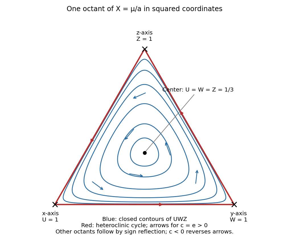
Phase portrait of one octant of the invariant sphere in normalized squared coordinates, with closed orbits and a heteroclinic boundary cycle
. Details. 
The equivariant Hopf theorem states that, under the usual nondegeneracy and transverse-crossing assumptions at an equivariant Hopf point, each complex axial isotropy subgroup of the spatial symmetry group combined with temporal phase produces a branch of periodic solutions with that spatiotemporal symmetry. Its common fixed-point space must have real dimension two, or complex dimension one. Restricting the Hopf normal form of a dynamical system to that plane gives a scalar complex amplitude equation; a nonzero real cubic coefficient provides a small periodic branch on the corresponding parameter side. The theorem supplies existence and symmetry, not stability.
Put and write , so . Three complex axial fixed lines areFor the first generator, its eigenvalues are , so the fixed line is exactly . Reflection supplies the conjugate line , representing the opposite rotation direction. For the other two generators, swapping coordinates, with or without the common minus sign, gives the displayed one-complex-dimensional fixed spaces.
These subgroups are inequivalent: the rotating-wave spatial projection has order three, while the standing-wave projections have order two; the two reflection types differ by the central phase , which conjugation cannot remove. Rotating the two standing lines by gives three orientations of each type, not new symmetry types. Therefore there are three distinct generic periodic branch types: rotating waves and two inequivalent standing-wave families. Their members have a period near , with the combined spatial–temporal operations determining their relative phase relations.
Common temporal phase requires a monomial in the first component to contain one more unbarred factor than barred factors. If the exponent differences for the two coordinates are , then . Equivariance under requires its spatial weight to be modulo three, hence . Up to degree five, gives times all quadratic and quartic polynomials in the intensities . The other possibility is , giving at degree five. No even-degree monomials satisfy the temporal weight.
Reflection determines the second component by exchanging indices. Thus the dihedral threefold Hopf normal form, through fifth order, iswith complex coefficients, at leading parameter order, and higher spatial-degree terms omitted. Coefficients may vary smoothly with the bifurcation parameter. The phase-sensitive quintic is allowed by the discrete threefold rotation, even though continuous independent rotations of the two coordinates would forbid it.
For a rotating wave, substitute . Its component amplitude and frequency obeyHere subscripts denote real and imaginary parts. For a standing wave, substitute , with . The resonant term becomes in the first component, and reflection ensures the second component agrees. ThereforeSet and . For constant leading coefficients, solving for givesSmooth parameter dependence adds common higher corrections but does not remove the generic difference between the two standing families. The rotating and standing component amplitudes differ already at cubic order unless their coefficient combinations accidentally agree. The standing waves have the same cubic amplitude, butwhich is generically nonzero. Thus all three branch types generically have different amplitudes, with the distinction between the standing families first visible at fifth order. In total Euclidean norm the rotating wave has amplitude , whereas each standing wave has amplitude . The relevant branches exist on the parameter sides making their small squared amplitudes positive; nonzero cubic coefficients are part of the generic Hopf assumptions.
Without the threefold rotation, a complex linear map need only commute with coordinate swapping and common phase. Commuting with makes its two diagonal entries equal and its two off-diagonal entries equal; common phase still forbids conjugate-linear terms. Thus the additional leading coupling iswhere is a small complex symmetry-breaking coefficient and a small common diagonal shift can be absorbed into . The old rotation forbade these off-diagonal entries because the two coordinates have different rotation weights. Further symmetry-breaking cubic and quintic terms are also allowed; retaining only the new linear terms describes the leading onset splitting.
In symmetric and antisymmetric coordinates , , the eigenvalues are and . With , the two primary Hopf thresholds and frequencies are thereforeThe reflection-preserving standing line remains invariant. The line also remains invariant because it is fixed by reflection combined with phase . Their generic periodic branches survive, now starting at separate thresholds when . If that real part vanishes, threshold coincidence is a nongeneric additional condition; frequency splitting may still occur.
The pure rotating-wave axes are not invariant: at the second equation has . Hence the old pure rotating-wave branches cease to be primary one-component branches from the origin. At fixed nonzero symmetry breaking, a simple Hopf onset has just the appropriate symmetric or antisymmetric mode. Away from the degenerate onset, normally hyperbolic rotating-wave periodic orbits may persist as mixed-mode periodic states with both components nonzero, paired by reflection. In common unfoldings such a pair is reached through a secondary reflection-breaking pitchfork bifurcation of periodic orbits from a standing branch. Its precise attachment, any folds, and stability depend on the nonlinear coefficients and cannot be fixed by symmetry alone.
The three rotationally conjugate orientations within each original standing family are no longer equivalent. Only the lines aligned with the surviving reflection symmetries are forced primary branches; other members can deform, pin to preferred orientations, or connect through secondary bifurcations. The generic bifurcation diagram thus replaces the coincident multi-branch Hopf onset by two separated simple Hopf onsets, removes the pure traveling-wave invariance, and unfolds the rotational degeneracies. This is the reflection-preserving splitting of a dihedral Hopf bifurcation; it does not by itself prescribe a unique global diagram.
Articles by others on the same topic
There are currently no matching articles.