The three contributions to the Frank elastic energy penalize distinct slow distortions of the nematic director. Nematic splay measures local spreading or convergence and is governed by . Nematic twist measures rotation around an axis perpendicular to the director, with cost . Nematic bend measures curvature of director integral lines; for a unit vector, , giving cost . These terms respect the head-tail symmetry of a nematic liquid crystal. Positive elastic constants oppose these distortions.
For the one-dimensional reduction assume lateral uniformity, so and depend only on . A prime below means . Directly differentiating the nematic director givesThe squared curl is . Subtracting the squared twist invariant givesConsequently the one-dimensional twisted nematic energy has elastic coefficientsA normal electric field has . There is a genuine factor-of-two inconsistency in the source: its initial functional places the electric term inside the overall factor , whereas its subsequent density and threshold use the full electric term. For the requested density and threshold, use the usual orientational coupling . Here is the dielectric anisotropy of a nematic, in the printed Gaussian-unit convention. If the first functional is instead read literally, this coupling is halved and the resulting threshold voltage is multiplied by .
Put and . Apply the Euler-Lagrange equations for two fields. Variation in , which does not appear explicitly, givesVariation in gives , orAt , , , and . With zero field, and satisfy both equations and the imposed azimuthal endpoints. Thus the quarter-turn planar texture is a stationary solution. Stationarity alone is not a claim of stability for arbitrary elastic constants.
To find the Fréedericksz transition, impose the additional strong planar anchoring . Write . The small-angle expansions areThe conserved and fixed total twist imply for a pure tilt perturbation. Linearizing the tilt Euler-Lagrange equation therefore givesSubstitute . A nonzero neutral amplitude requiresSince , the quarter-turn nematic instability threshold isThis is the first zero-endpoint mode: higher sine modes replace by and cost more elastic energy. The quadratic energy change is , so the first mode has negative stiffness above this voltage. The result assumes and . If the latter is negative the planar state is already unstable at zero field; for negative dielectric anisotropy of a nematic, a normal field opposes this tilt. The literal initial electric prefactor would give .
For reflective operation of the twisted nematic field effect, orient each polarizer's transmission axis along the adjacent planar nematic director. Light entering through the top polarizer initially has linear polarization. At low voltage, adiabatic optical following in a twisted nematic rotates it through a quarter turn to as it travels downward, so it passes the bottom polarizer and reaches the mirror. On returning, it follows the reverse twist back to and exits the top polarizer: the pixel appears bright. At sufficiently high voltage, positive dielectric anisotropy of a nematic aligns most of the director with the normal field. The bulk no longer produces the quarter-turn optical rotation, so the crossed bottom polarizer blocks the incident light and the pixel appears dark. Elastic relaxation restores the bright twisted state after voltage is removed. The adiabatic requirement is more precisely , involving birefringence, not thickness alone. Voltage switches director orientation and hence the reflected brightness; it does not require the liquid crystal to emit light.
Set and . Multiplying the Langevin equation by and integrating givesThe expected value of is zero. For the printed dot-product force covariance, write , so . Without any white-noise approximation the trace variance isThe intended short-correlation approximation replaces by , where is the Dirac delta. It requires the force correlation time to be much shorter than and the observation time. ThenAt thermal equilibrium, the equipartition theorem gives . Taking the long-time limit determines the vector noise normalization in inertial Langevin dynamics:This factor six corresponds to the dot-product covariance across three components. If were defined for one component instead, its integrated strength would be before dividing by , and the acceleration strength would be .
Finite rapid correlation is not literally a Dirac delta. For a stationary force and local drag, its exact limiting velocity trace isThis follows by splitting the double convolution into and . Thus equipartition fixes the weighted integral, not just , unless the short-correlation approximation is made. For example, gives . The remaining explicit formulae use the intended continuous-time Gaussian white noise limit.
Assume isotropic jointly Gaussian noise, as appropriate to an isotropic bath. The component covariance isThe scalar moment identities in the question must now be applied to a fixed Cartesian component , not to the magnitude of the vector. Its variance isIn the -fold integral for , the Isserlis theorem replaces the force product by a sum of complete pairings. Each pairing yields identical two-time integrals, hence . Pair the first labelled factor in ways, then the first unpaired factor in ways, and continue. The Gaussian even-moment pairing count isOdd force products vanish, soFor completeness, summing the scalar moment-generating function givesThe same Gaussian process argument for every linear combination of components gives the vector characteristic function . Inverting this Fourier transform yields the normalized multivariate Gaussian distributionThe initial condition is a velocity Dirac delta as , and the long-time limit is the thermal velocity density. The converted TeX's exponent is damaged; the PDF has the squared norm displayed here. The scalar pairing formula cannot be interpreted as a vector-norm formula: the radial moments of an isotropic Gaussian vector instead give in three dimensions.
Integrate the velocity once more. Interchanging the time integrals gives the integrated Ornstein-Uhlenbeck displacementFor the stated fixed initial position and velocity,Let and . Its component covariance comes from integrating the squared noise kernel:Therefore the total centered variance isThe mean-square displacement from additionally contains . Confusing this deterministic drift contribution with centered variance changes the short-time conclusion.
For times longer than the force correlation time but , the mean motion is and the centered trace is . Thus a nonzero fixed initial velocity produces a leading ballistic mean-square displacement ; conditioned on , the white-noise displacement variance instead starts as . If one averages over an independent equilibrium initial velocity, its covariance adds , givingThis is the usual thermal ballistic regime, before velocity memory has relaxed. At , the conditional mean approaches , while the centered trace is . Its leading behavior is diffusion with and , as successive displacement increments lose inertial memory. At times below a finite force correlation time the white-noise short-time expansion is not applicable; for a regular force covariance and fixed initial velocity the leading noise-induced displacement variance is of order .
The filament bending modulus has units force times length squared. The perpendicular drag coefficient in this equation is drag per unit length divided by velocity, so its units are force times time per length squared. Hence has units length to the fourth power. Balancing oscillatory viscous drag against elastic force density gives the elastohydrodynamic penetration lengthIncreasing frequency confines the response nearer the actuator. The chosen coefficient one in this characteristic length is a convention; the exact decay lengths acquire the root-dependent factors found below.
The overdamped filament bending equation is linear, so sinusoidal forcing has a sinusoidal steady response at the same frequency. Write with . Substitution givesUsing the elastohydrodynamic penetration length from the previous part reduces this ordinary differential equation toThe boundary conditions become , , and decay of and its derivatives at infinity. The derivative condition expresses zero bending moment at the driven end, rather than a clamped slope. This separation of variables constructs the periodic response; an unspecified initial shape can add a transient solution of the homogeneous evolution problem.
Set . The characteristic polynomial is , whose roots have arguments , , , and . Only the last two have negative real part and decay at infinity. Write and ; the admissible roots areThus . Since , the boundary equations are and . ThereforeTaking real parts gives the oscillatory bending of a moment-free semi-infinite filamentThe first phase is constant along paths with , so that contribution travels left. The second has and travels right. Both are forced, attenuating patterns in an overdamped medium; they are not undamped inertial waves. Their amplitudes are equal at the driven end, but gives decay lengths and . Hence the right-travelling contribution dominates away from the end, because it decays more slowly; its amplitude relative to the left-travelling one grows as .
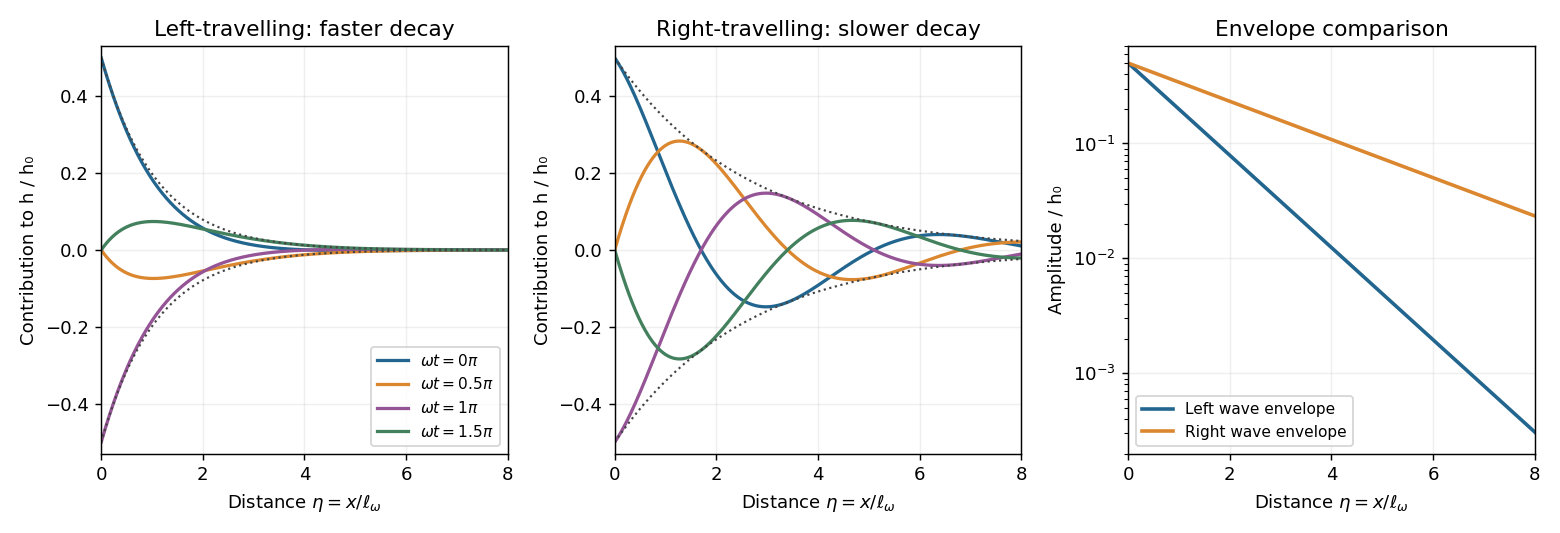
Counter-propagating contributions to a driven filament, with faster attenuation of the left-travelling wave
. Details. 
The envelopes in the sketch show this amplitude comparison independently of the instantaneous phase. At particular points a cosine can vanish or the two terms can interfere, so dominance refers to envelopes and the far-field response, not to a strict pointwise inequality at every time.
Use the arc length and the unit tangent of an inextensible filament. In the high-force state choose its positive longitudinal branch. The constraint givesThe extension is . The curvature of a space curve obeys . Since is second order in small fluctuations, its squared contribution is fourth order. Thus the worm-like chain energy through quadratic order isPositive force suppresses transverse orientation fluctuations, while the filament bending modulus penalizes their spatial variation.
To apply the equipartition theorem without missing either component or a mode-counting factor, expand each component in a real orthonormal basis of eigenfunctions of , , with and . The quadratic energy is . Each real quadratic degree of freedom contributes , soFor a chain long compared with the force-dependent correlation length, the interior is translation invariant and the mode sum per length becomes . Equivalently, for the Fourier transform ,The negative and positive wavenumbers here represent the real-field mode count consistently, rather than two independent complex modes. Summing both transverse components gives the high-force worm-like chain elasticitywhere the integral follows by setting and using . ThereforeHere is the three-dimensional zero-force persistence length. The result requires , negligible backbone stretching, and a long-chain bulk approximation. It does not describe the eventual bond-stretching regime. For a continuum polymer description, the force-dependent length should also exceed the microscopic cutoff.
For comparison, a three-dimensional freely jointed chain has contour length and independent link orientations. At force , a link of polar angle has Boltzmann factor with . Its angular canonical partition function isThe total canonical partition function is . Differentiating with respect to force gives the force-extension of a three-dimensional freely jointed chain:ConsequentlyThe extension deficits scale as and respectively. Inverting them gives force divergences proportional to the first and second inverse powers of the deficit. Freely jointed link rotations cost no bending energy; the worm-like chain instead has a continuum of coupled bending modes whose contributing wavelengths change with force. Setting a long-wavelength coarse-grained link length can match weak-force statistics, but does not make these high-force laws identical.
For the transverse tangent correlation of a stretched worm-like chain, use a separation consistently: the source writes but integrates a separation denoted . In the translation-invariant bulk the spatial average is redundant andTo evaluate the integral without an assumed decay law, let be the inverse Fourier transform of . Then . Away from zero, decay at both infinities requires with . Integrating across zero yields , so . ThusAt this agrees with the two-component equipartition theorem calculation. The correlation length decreases with force and is distinct from the zero-force persistence length. The full tangent correlation has a nonzero aligned background; the exponentially decaying quantity here is specifically the transverse correlation.
For a finite open chain, the source's integral samples beyond and supplies no endpoint tangent conditions. An exact finite-length correlation is therefore not uniquely specified. The result above is the intended bulk form when . As one explicit finite convention, periodically extending the tangent fluctuations gives the periodic finite-length tangent correlation of a stretched worm-like chainwhere is the distance from zero around the periodic interval. Then , and the extension formula acquires this same finite-length factor. The bulk law is recovered as . This makes the endpoint assumption explicit rather than claiming an unspecified finite-chain correlation is exactly translationally invariant.
Articles by others on the same topic
There are currently no matching articles.