Past exam of the mathematics course of the University of Cambridge / 2010 / iii / Paper 61 (Planetary System Dynamics)

Put $\mathcal{G}=G(M_{\star }+M_{\mathrm{pl}})$, $h=\sqrt{\mathcal{G}a(1-e^2)}$, $\theta =\omega +f$ and $L=n_{\mathrm{pl}}t$. Here $h$ is the specific angular momentum, $f$ is the true anomaly and $\omega$ is the planar longitude of periapsis. Differentiating the Kepler orbit equation with $\dot{f}=h/r^2$ givesResolve the velocity along the radial and tangential unit vectors, $\hat{\mathbf{r}}=(\cos \theta ,\sin \theta )$ and $\hat{\mathbf{\theta }}=(-\sin \theta ,\cos \theta )$. The identities $\sin f\cos \theta -\cos f\sin \theta =-\sin \omega$ and $\sin f\sin \theta +\cos f\cos \theta =\cos \omega$ yieldThis is the Kepler velocity hodograph: the velocity runs around a circle whose centre is displaced by the orbital eccentricity.

The centre of mass condition gives the star's barycentric position ${\mathbf{r}}_{\star }=-\mu a_{\mathrm{pl}}(\cos L,\sin L)$. Translating to the star without rotating the axes gives ${\mathbf{r}}^{\prime }=\mathbf{r}-{\mathbf{r}}_{\star }$ and ${\mathbf{v}}^{\prime }=\mathbf{v}-{\dot{\mathbf{r}}}_{\star }$. From Kepler's third law, $n_{\mathrm{pl}}^2{a}_{\mathrm{pl}}^3=\mathcal{G}$, soConsequentlyThe small displacement and the larger reflex velocity have different orders: $|{\mathbf{r}}^{\prime }-\mathbf{r}|/a=\mu \alpha$, but the reflex speed divided by the circular speed is $\mu {\alpha }^{-1/2}$. These are the source of the astrocentric osculating-element oscillations.

For the coordinate ratio, the exact result isFor fixed $e<1$, $r/a\ge 1-e$, so this is $O(\mu \alpha )$ on any angular region with $|\cos \theta |$ bounded away from zero. The printed coordinate claim is not uniform over a full orbit: at $x=0$ its ratio is undefined. The nonsingular statement is $|{\mathbf{r}}^{\prime }-\mathbf{r}|/r\le \mu \alpha /(1-e)$, assuming the pericentre distance remains much larger than the binary separation.

Squaring the two components of the velocity givesAt $\mu =0$, $\kappa =0$ and $\mathcal{G}=G{M}_{\star }$. Sincethis reduces to the vis-viva equation, $v^{\prime 2}=G{M}_{\star }(2/r-1/a)$.

Now let the barycentric Kepler orbit be circular, write $\Delta =L-\theta$ and $\epsilon =\mu {\alpha }^{-1/2}\ll 1$, and put $v_0=\sqrt{\mathcal{G}/a}$. The osculating orbital elements about the star use the gravitational parameter $G{M}_{\star }=(1-\mu )\mathcal{G}$. To the required order, $r^{\prime }=a[1+O(\mu \alpha )]$ and $v^{\prime 2}=v_0^2[1+2\epsilon \cos \Delta +O({\epsilon }^2)]$. The specific orbital energy therefore impliesHere $\mu =o(\epsilon )$ and ${\epsilon }^2=o(\epsilon )$ under the stated hierarchy. Even at a phase where the leading cosine vanishes, the absolute error bound remains valid.

Finally, use the eccentricity vector ${\mathbf{e}}^{\prime }=({\mathbf{v}}^{\prime }\times {\mathbf{h}}^{\prime })/(G{M}_{\star })-{\hat{\mathbf{r}}}^{\prime }$. In radial and tangential components it isThe translation changes the radial basis only by $O(\mu \alpha )$, whereas $v_r^{\prime }=-v_0\epsilon \sin \Delta +O(v_0\mu \alpha )$ and $v_{\theta }^{\prime }=v_0(1+\epsilon \cos \Delta )+O(v_0\mu \alpha )$. ThusFor the original circular Kepler orbit, $\omega$ and $f$ are separately arbitrary; their sum $\theta$ is well defined. Using the eccentricity vector avoids introducing an undefined pericentre for that circular Kepler orbit.

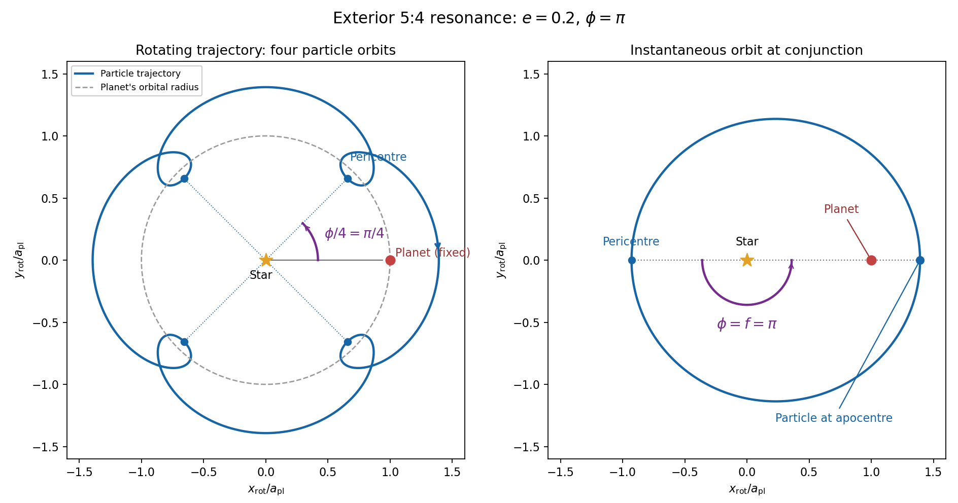
Use $s=p+1$ and the exterior mean-motion resonance condition $s{n}_r=p{n}_{\mathrm{pl}}$. Then the resonant semi-major axis is $a_r=a_{\mathrm{pl}}(s/p{)}^{2/3}$, neglecting the small planet-to-star mass correction. For the geometric construction, take $a_{\mathrm{pl}}=n_{\mathrm{pl}}=1$, $p=4$, $e=0.2$, $\varpi =\pi /4$ and start the particle at pericentre. Solve Kepler's equation $M=E-e\sin E$ with $M=(4/5)t$. Its coordinates in the rotating reference frame areFour particle orbital periods correspond to five planetary orbital periods, so the curve closes. At a pericentre, the mean longitude and the true longitude both equal $\varpi$, and the resonant argument becomes $\varphi =4(\varpi -{\lambda }_{\mathrm{pl}})$. Thus the four pericentre directions are $\varphi /4$ modulo $\pi /2$. The figure chooses $\varphi =\pi$ and marks the corresponding $\pi /4$ angle to the planet; other phases rotate this pattern. Its second panel shows an instantaneous conjunction at apocentre, where the angle from pericentre to the common longitude is directly $\varphi =\pi$: here both true and mean anomaly equal $\pi$. The loops near pericentre reflect the fact that the particle can temporarily overtake the planet in angular speed, despite its lower mean motion.

For the evolution equations, $\lambda$ must be the mean longitude. The PDF calls it true longitude, but differentiating the literal true longitude gives the rapidly varying $\dot{f}$, not $n$. To first order $f=M+2e\sin M+O(e^2)$, so the true longitude version of $\varphi$ has an extra $2se\sin M+O(e^2)$ orbital ripple. The stated Lagrange planetary equations and slow complex eccentricity equation are interpreted consistently as orbit-averaged equations in mean longitude. The pericentre geometry of an exterior resonance above is unchanged by this distinction.

Let $F_r,F_{\theta }$ be perturbing forces, and let $m$ be the particle's mass. The angular momentum about the star satisfiesThe central gravitational force and the radial perturbation have zero torque. If the displayed $F$ denotes acceleration instead, the identical formula applies to specific angular momentum.

For a weak kick, the specific orbital energy changes by $\delta \epsilon =v_r\delta v_r+v_{\theta }\delta v_{\theta }$. A planet leading the particle pulls it forwards, while a trailing planet pulls it backwards. For a nearly circular exterior Kepler orbit, a forward tangential kick raises angular momentum and semi-major axis, lowers mean motion, and makes the next conjunction occur sooner in the synodic cycle. Its longitude retreats relative to the unperturbed conjunction sequence. A backward kick produces the opposite shift. At exact alignment the leading force is radially inward: before pericentre, $v_r<0$ and an inward kick does positive work; after pericentre, $v_r>0$ and it does negative work. These likewise raise or lower semi-major axis. At an apsis, a purely radial infinitesimal kick has no first-order energy change but changes the eccentricity vector, so angular momentum alone does not determine every timing change.

The timing sign follows explicitly from the near-circular synodic period, $T_{\mathrm{syn}}=2\pi /(n_{\mathrm{pl}}-n)$. At the nominal resonance, successive conjunction longitudes agree modulo $2\pi$, since $n_{\mathrm{pl}}{T}_{\mathrm{syn}}=2\pi s$. A persistent small change givesThis is the accumulated mean timing shift; an actual impulsive encounter can also change the instantaneous orbital phase and longitude of periapsis.

Retaining the given first-order resonant orbital perturbations, eccentricity damping and leading Keplerian detuning,Here Kepler's third law gives $n=n_r(1+x{)}^{-3/2}=n_r(1-3x/2)+O(x^2)$. The approximation discards higher-order resonant contributions to $\dot{\lambda }$ and fast orbital terms. Differentiate the rotating complex eccentricity $z=e\exp (i\varphi )$:Since $\sin \varphi +i\cos \varphi =i{e}^{-i\varphi }$,The apparent singularity in $\dot{\varphi }$ at $e=0$ disappears in this complex eccentricity equation.

Take $A>0$, and the conventional positive resonant coefficient $C>0$. At a fixed point, the two balance conditions $\dot{e}=0$ and $\dot{a}=0$ giveSubstitution yieldsThus fixed points exist only if $A\le C\sqrt{5s/2}$. With strict inequality, put $S=\sqrt{(5/2)s{C}^2-A^2}$ and ${\psi }_f=\arctan (A/S)\in (0,\pi /2)$. Thenrespectively. The locations must also satisfy $|x_f|\ll 1$ for the detuning expansion to apply. At equality the phases merge at $3\pi /2$ and $x_f=0$. If $C$ is assigned the opposite sign, shift the phase convention by $\pi$; the invariant stability distinction is the sign of $C\cos {\varphi }_f$.

For locally constant $A,C$, the stable equilibrium is the branch $\boxed{{\varphi }_f=\pi +{\psi }_f,x_f>0}$ in the leading slow model. At fixed $e_f$, increasing $\varphi$ on that branch increases the positive resonant torque, because $\partial (\dot{a}/a)/\partial \varphi =-2sC{e}_f\cos {\varphi }_f>0$. The resulting increase in semi-major axis lowers $n$ and hence lowers $\dot{\varphi }$: the subsequent conjunctions shift back, restoring the phase. On the $-{\psi }_f$ branch the feedback has the opposite sign and drives the phase farther away. Eccentricity damping removes the oscillatory disturbance on the restoring branch.

One can verify that this feedback stabilizes the coupled variables rather than just the phase. Treat $A,C$ as locally constant, and write $z=u+iv$. Then $\dot{u}=-Au+Bxv$, $\dot{v}=-C-Av-Bxu$ and $\dot{x}\simeq -2sCv-4A/5$. At a fixed point $Bxv=Au$. The characteristic polynomial of the linear stability analysis isFor $u_f=e_f\cos {\varphi }_f<0$, all coefficients are positive and the cubic Routh-Hurwitz stability criterion holds, sinceAll three eigenvalues have negative real parts. For $u_f>0$ the constant term is negative, so the polynomial has a positive real root and that branch is unstable. The merged case has a zero eigenvalue. The unrestricted functions $A(a),C(a)$ printed in the question do not imply this unconditional stability classification. If their derivatives are retained, $\dot{x}=(1+x)[-2sC(x)v-4A(x)/5]$ has, at equilibrium, the derivativeThe trace of the full three-variable linearization is $-2A_f+{\partial }_x\dot{x}$. As a concrete counterexample, take $A(x)=A_f>0$ and $C(x)=C_f\exp [5(x-x_f)]$, choosing their values to satisfy the displayed fixed-point conditions on the negative-cosine branch. Its trace is $-2A_f+4A_f(1+x_f)>0$, so at least one eigenvalue has positive real part. Both coefficients are smooth. Thus the restoring conjunction feedback identifies the stable branch of the usual locally constant model, but additional assumptions on coefficient variation are necessary to assert stability for every allowed function.

For a circular orbit the origin of mean anomaly is arbitrary because there is no distinguished pericentre. Choose $M=0$ at the ascending node, so $M$ is also the argument of latitude. If a different periapsis convention is used, replace $M$ below by $M+\omega$. The orbital-frame rotation from inclination and node givesIn particular the crossing at $M=0$ has increasing $z$ for prograde $n>0$ and $0<I<\pi$, confirming the ascending node convention.

Put $ϵ=a/a_{\mathrm{pl}}$ and $c=\cos \psi =\hat{\mathbf{r}}\cdot {\hat{\mathbf{r}}}_{\star }$. The binomial series expansion of the direct disturbing function isThe indirect disturbing function subtracts $G{M}_{\star }ac/a_{\mathrm{pl}}^2$, cancelling the dipole term. The constant $G{M}_{\star }/a_{\mathrm{pl}}$ has no spatial derivative and does not perturb the particle. After omitting that constant, the leading stellar quadrupole disturbing function isThus the PDF's equality is understood modulo a dynamically irrelevant additive constant and higher multipoles.

Define $\ell =M+\Omega$ and let ${\ell }_{\star }$ be the star's orbital longitude as seen from the planet. Its orbital plane has $I_{\mathrm{pl}},{\Omega }_{\mathrm{pl}}$. The vector from planet to star is the negative of the planet's heliocentric vector: if ${\ell }_{\mathrm{pl}}$ describes that latter vector, use ${\ell }_{\star }={\ell }_{\mathrm{pl}}+\pi$. This sign matters in $\cos \psi$ but drops out of ${\cos }^2\psi$. Expanding the two rotated unit vectors givesFor example, the particle's horizontal correction is $-(I^2/2)\sin (\ell -\Omega )(-\sin \Omega ,\cos \Omega )$, while its vertical component is $I\sin (\ell -\Omega )$; their dot products with the corresponding stellar components produce these terms. No cubic terms occur because simultaneous reversal of both small orbital inclinations leaves the dot product unchanged.

The two mean longitudes are uniform for the circular Kepler orbits, so orbit averaging is uniform in both $\ell$ and ${\ell }_{\star }$. Set $c_0=\cos (\ell -{\ell }_{\star })$ and $c_2=\cos \psi -c_0$ through quadratic order. The needed averages follow by integrating sine and cosine products over $[0,2\pi {]}^2$:For the last identity, expand $c_0=\cos \ell \cos {\ell }_{\star }+\sin \ell \sin {\ell }_{\star }$ and factor the two integrations, each using $⟨{\sin }^2\ell ⟩=⟨{\cos }^2\ell ⟩=1/2$. Squaring $c_0+c_2$ now yieldswhere the error includes all fourth-order combinations of the two orbital inclinations. ThereforeMultiplying this by $G{M}_{\star }{a}^2/a_{\mathrm{pl}}^3$ gives the requested secular disturbing function. Equivalently, the exact angular factor for two circular rings is $(3{\cos }^2{I}_m-1)/8$, where $I_m$ is their mutual inclination; its small-angle expansion gives the same result. This is the double-averaged circular tidal potential.

For aligned equatorial and planetary orbital planes, set $I_{\mathrm{pl}}=0$. The secular stellar quadrupole disturbing function then has derivative ${\partial }_I{\overline{\mathcal{R}}}_{\star }=-3G{M}_{\star }{a}^{2}I/(4a_{\mathrm{pl}}^3)$. The supplied Lagrange planetary equations for nodal precession givesThe planetary quadrupole coefficient $J_2>0$ contributes ${\partial }_I{\overline{\mathcal{R}}}_{J_2}=-3G{M}_{\mathrm{pl}}{J}_2{R}_{\mathrm{pl}}^{2}I/(2a^3)$, henceBoth are retrograde nodal precession rates. Equating them cancels $n$ and gives the Laplace radiusThe planetary quadrupole dominates inside $a_L$ and the stellar tide outside it. These are small-inclination rates for planet-bound Kepler orbits in the hierarchical regime $a\ll a_{\mathrm{pl}}$. At exactly $I=0$, the node itself is undefined; the rates are the limiting precession frequencies of an infinitesimal tilt.

Assume the physical coefficients $Q_a,Q_b$ are positive. Differentiate the catastrophic disruption threshold:The bracket is strictly increasing from a negative value to positive infinity, so there is one critical point and it is the global minimum. In fact $Q_D^{\ast }$ tends to infinity at both endpoints $D\to 0$ and $D\to \infty$. The strength-gravity disruption transition is thereforeAt this diameter, $b{Q}_b{D}_w^b=a{Q}_a{D}_w^{-a}$, so $Q_w^{\ast }=[(a+b)/b]Q_a{D}_w^{-a}$. This minimizes the full catastrophic disruption threshold; it need not be where its two contributions are equal.

For equal-density spherical planetesimals, the specific impact energy per unit target mass is $\frac{1}{2}(D_{\mathrm{im}}/D_w{)}^3{v}_{\mathrm{rel}}^2$. Setting this to $Q_w^{\ast }$ gives the catastrophic projectile diameterHere $v_{\mathrm{rel}}$ is the impact speed, the threshold is defined per target mass, and energy-coupling changes are not included. If projectile and target densities differ, multiply the diameter by $({\rho }_{\mathrm{target}}/{\rho }_{\mathrm{projectile}}{)}^{1/3}$. For $a=1/2$, $b=3/2$,so collecting the powers givesThe result presumes that this projectile diameter is available in the population.

For the dust, $n(D)dD$ is the total number in a diameter interval, not a number per unit volume. The mass normalization of a power-law size distribution with dust mass $M/2$ givesThe approximation uses $(D_{\min }/D_{\max }{)}^{4-\alpha }\ll 1$. Merely having a small diameter ratio does not guarantee this accuracy if $\alpha$ approaches four, so retain the exact denominator in that case.

With $\gamma >0$, the stated Poynting–Robertson drag law integrates directly:Thus dust arrives in order of increasing diameter. This is burst transport under inverse-size radial drag, assuming an instantaneous release at $r_0$ and no intervening destruction or changes of diameter.

Dust that reaches the planet's orbital radius has several possible fates. It can pass without a close encounter and continue spiralling towards the star; undergo resonant trapping of dust in an exterior mean-motion resonance, where resonant torque temporarily balances the drag; be scattered onto a different stellar Kepler orbit or ejected; or collide with the planet and be accreted. Resonant trapping of dust can increase orbital eccentricity until escape or an encounter becomes possible. Temporary planet-bound capture can become permanent if drag or another dissipative process removes sufficient energy. Arrival at a radial circle alone does not guarantee a collision with the planet at the correct longitude.

A more massive planet has a larger Hill sphere, stronger resonant perturbations and stronger planetary scattering. Capture into a mean-motion resonance is favoured when drift across it is slow compared with its libration timescale. Since $|\dot{r}|\propto D^{-1}$ here, larger grains drift more slowly and are generally easier to trap; small fast-drifting grains more readily cross a resonance. Grain radiation pressure can also move resonance locations, though the prescribed nearly circular drift model omits that additional change. For direct impact, a larger physical radius increases the geometric cross-section, and gravitational focusing gives, in the two-body encounter approximation,A compact massive planet can nevertheless scatter or eject grains rather than hit them: its encounter region can be much larger than its physical radius. Slower dust migration permits more repeated encounter opportunities. These competing effects mean neither planet mass nor grain diameter alone specifies an accretion probability.

For the idealized complete-accretion calculation, put $T=t_p(D_{\max })$ and $\eta =D_{\min }/D_{\max }$. At time $t$, the arriving diameter is $D_t=D_{\max }t/T$ and $d{D}_t/dt=D_{\max }/T$. Hence the dust-burst accretion pulse follows from the arriving mass per diameter:Dropping the small lower-cutoff normalization correction gives the requested expressionThe rate is zero before the smallest grains arrive and after the largest arrive. Integrating the exact expression over its support returns $M/2$, as required by mass conservation. The approximate expression has that integral to the same lower-cutoff accuracy. This pulse assumes no resonant delay or scattering loss before accretion.

For the surface density of a size-sorted dust burst, take $0<r<r_0$ and writeAt fixed $t>0$, the size-radius map is monotone and $d{D}_r/dr=2r{D}_r/H_r$. Define $\Sigma (r,t)$ as the azimuthally averaged surface density, so the mass in an annulus is $2\pi r\Sigma dr$. Transforming the power-law size distribution into radial mass givesIt follows thatThe requested leading approximation omits $1-{\eta }^{4-\alpha }$ from the denominator. The surface density is zero where the inferred $D_r$ lies outside the original size interval. Equivalently, one can obtain it from the instantaneous inward mass flux divided by $2\pi r|\dot{r}(D_r)|$. At $t=0$ the idealized initial distribution is a delta-function ring at $r_0$; the formula above describes the subsequent radial spread. No uniform initial azimuthal distribution is required for this azimuthal average, but the local density of a clump would require its angular evolution. If the complete-absorption planet assumption is retained, this expression holds exterior to $r_p$ and $\Sigma =0$ interior to the planet.