Write and . When the ice sphere grows by volume , it consumes liquid volume . The difference is expelled from the fixed cavity. Thus mass conservation fixes the outward Darcy flux in the surrounding porous medium:The Darcy law and implyMatching at the cavity wall, whose internal pressure is uniform, givesThe solid and liquid pressures are equal when the Gibbs--Thomson relation is neglected; nevertheless the coexistence temperature changes with their common pressure because their specific volumes differ. Along coexistence, equality of chemical potentials givesHence the common-pressure melting-point slope is . To first order in the pressure change,The multiplying this coefficient is absolute temperature, approximately for water; a temperature difference may equally be measured in kelvin or degrees Celsius. Substituting the numerical value from the Celsius scale into a thermodynamic denominator would be incorrect.
In the quasi-stationary thermal conduction approximation, neglect advective heat transport and use the stated effective conductivity outside the sphere. The radial Laplace equation gives the bounded solid temperature and the liquid/porous-region temperature:This treats the exterior as a uniform conducting medium, as required by the printed reduction; distinct cavity and porous-medium conductivities would give an additional thermal resistance. There is no solid-side heat flux in the bounded quasi-stationary solution. The Stefan condition therefore becomesEliminate and to obtainFor , and , this isThe pressure follows either from the Darcy flux or the Stefan condition:In particular : rising pressure progressively reduces the available undercooling. This is spherical freezing inside a porous cavity, whose fixed hydraulic outlet radius distinguishes it from freezing directly through a porous matrix.
For the idealized zero-radius start, integration givesA finite seed replaces the right side by its difference from the initial value. The reduction ends when the sphere fills the cavity.
For , hydraulic drainage is easy and the pressure feedback is small throughout the cavity. The leading expressions areThis is ordinary conduction-controlled spherical solidification, with a completion time asymptotic to .
For , distinguish the initial crossover from the pressure-dominated regime. At , equivalently , the same square-root growth applies and . At , equivalently ,The interface approaches , the pressure approaches the finite coexistence value , and growth becomes hydraulically limited. The leading completion time is . The cube-root approximation is not valid at the instant of nucleation, where the initial square-root regime must be retained.
Use the one-sided thermal conduction model encoded by the requested dispersion relation: neglect solid-side perturbation heat flux, take equal phase densities, and let the normal point from solid into liquid. Write the isotropic linear kinetic undercooling law using the solidification attachment mobility :Here is solid-liquid surface energy, is the sum of principal curvatures, and is absolute temperature. Positive curvature convex into liquid lowers the equilibrium freezing temperature through the Gibbs--Thomson relation. The planar base state has .
Set and defineThe paper's is the latent-to-sensible heat ratio, the reciprocal of the common Stefan number convention. Below, velocities, lengths and growth rates are dimensionless in these scales. In the travelling coordinate , the liquid heat equation gives , while the bounded solid steady field is constant. Matching a decaying liquid profile to the Stefan condition givesThe kinetic undercooling condition is . ThusThe speed is constant for , determined by and the attachment coefficient in the specified scales. Thermal diffusivity sets the exponential decay length , not the selected speed. Including solid-side perturbation conduction would change the stability equation below.
For linear stability analysis, corrugate the interface to and write the liquid perturbation as . The liquid heat equation requiresFor this graph the linearized curvature is . Evaluate the temperature on the displaced interface: its perturbation is . The kinetic undercooling law therefore givesLikewise the derivative evaluated at the displaced surface is , with . The Stefan condition at perturbation order readsElimination proves the one-sided kinetic solidification dispersion:The destabilizing term comes from a protrusion encountering colder liquid; capillarity and kinetic relaxation oppose it.
At , and the base liquid has no thermal contrast generated by latent heat. The interface obeys : positive surface energy damps all nonzero modes, while is neutral at this order. Here the thermal perturbation amplitude vanishes, so the auxiliary decay exponent is immaterial to that pure kinetic relaxation. At , and the formal limit givesFor it has a negative real branch and no growing branch; at the interface branch is neutral. Strictly, is a singular endpoint of the travelling profile: no finite-width stationary exponential connects to the far-field value zero. These stability statements describe the limit of the travelling-front model.
For , assume at small wavenumber. ExpandSubstituting into the dispersion relation cancels on both sides and givesAt the capillary stability threshold for a kinetic freezing front , continuing the same expansion gives : the nonzero long waves are damped even at threshold.
For large wavenumber, multiply the dispersion relation by and eliminate using the thermal equation. The exact algebraic form isIt prevents the uncontrolled replacement when itself is of order . In the usual small-capillarity range the leading results areFor the second result, set in the cubic; its quadratic-order balance gives . Thus positive capillarity stabilizes sufficiently short waves. If also and , the useful reduced approximation isits finite terms should not be treated as a uniform expansion for arbitrary fixed .
For completeness, large dimensionless capillarity has different balances. At , and . For , , so . At , the real branch reaches : for its growth rate is , and for that endpoint is exact. For at this boundary, or for , the selected real- normal mode ceases to exist at sufficiently large wavenumber; the full diffusion problem includes a thermal continuous spectrum and cannot be assigned a real isolated interface growth rate by this ansatz there. Indeed, writing the bulk thermal perturbation as reduces its heat equation to , whose half-line diffusion modes have decay rates for . The thermal branch endpoint is . Loss of a damped isolated interface mode is not a morphological instability.
The approximate instability condition is already clear from the long-wave coefficient: , equivalently . In fact it is exact for growing modes of the present one-sided model. At , let , so . The right side of the dispersion relation becomesFor real , the residual is strictly increasing, sinceTherefore a unique positive root exists precisely when . For , the unstable band isThere are no unstable oscillatory roots hidden by this real-root test. Indeed, if and , the thermal equation implies . For , the imaginary parts of the two equations would require , contradicting . Thus growing modes have real and real .
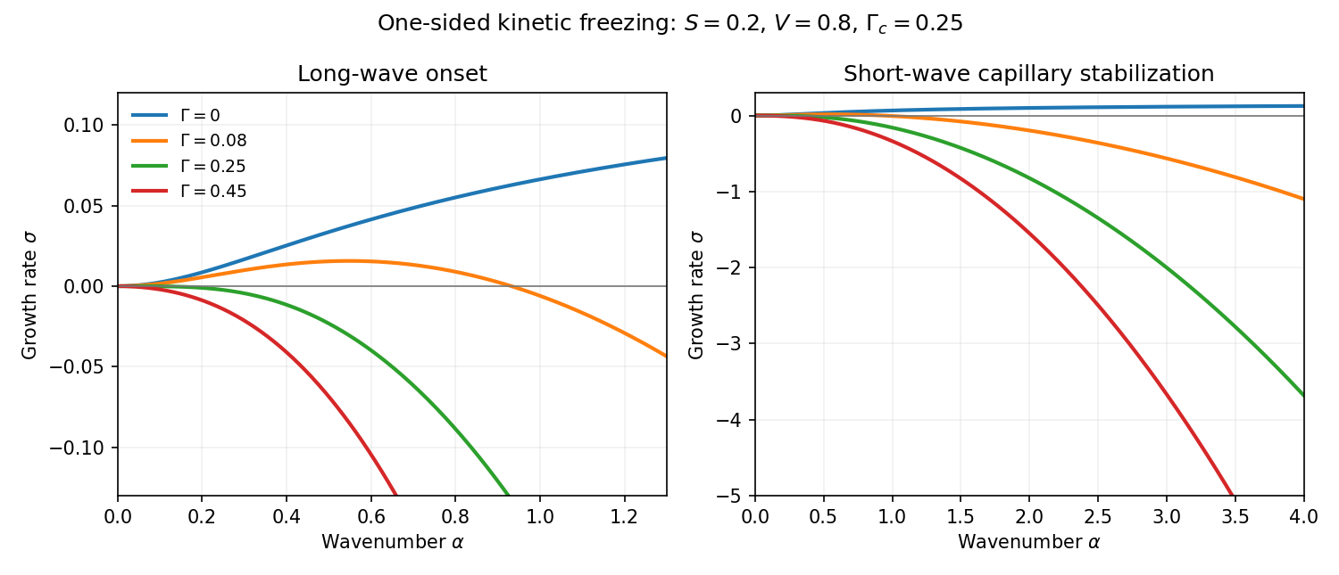
The sketch shows zero capillarity approaching the positive plateau , weak capillarity giving a positive band followed by short-wave damping, and threshold/stronger capillarity giving damping at every nonzero wavenumber. The zero-wavenumber mode is a translation. As with fixed positive , both the unstable bandwidth and the positive growth rates shrink to zero; the small-wavenumber expansion is not uniform in that limit.
Use a one-sided top-hat plume model with Boussinesq approximation and neglect the solid/liquid density difference in the interfacial volume source. Define the positive ablation speed , volume flux per unit wall span , and kinematic momentum flux . Let ambient entrainment per height be , with entrainment coefficient , and take for the salinity contribution to density. Conservation of volume and vertical momentum, with negligible wall stress and negligible vertical momentum of entering fluid, givesOnly the ocean-facing edge entrains. Using two edges would change the entrainment coefficient in these formulas.
To derive the heat balance, choose liquid specific enthalpy and solid specific enthalpy . A horizontal slab receives ambient volume with enthalpy , and solid mass-equivalent volume with enthalpy . ThusSubtract and divide by :Similarly, the incoming salt flux is , so . Subtracting provesBoth anomalies are negative for fresh, cold melt entering the ocean. These balances account for the heat needed to melt the entering ice, rather than treating it as already-liquid water at .
Now use , the large latent-to-sensible heat ratio convention of the paper. Put . The stated small plume-deficit limits allow us to replace plume by their ambient values in the diffusive interfacial fluxes. The Stefan condition and interfacial salt balance are thenFor the compositional Péclet number , solve the second equation and impose the liquidus:Substitution in the heat balance gives the diffusive glacier-ablation interface lawHere is the liquidus slope, unrelated to the surface-energy parameter of the previous question. If , and , the physical root isIt is positive when , exactly the condition that the ocean is warmer than its own liquidus. Since and ambient properties are fixed, is constant with height in this approximation.
For the melting-driven saline wall plume, measure height from a virtual origin. The integrated anomaly balances areIn the specified small-deficit regime the meltwater volume is negligible compared with entrainment. Indeed, the solution below gives , so a small compositional plume deficit implies . Thus retain for the leading power laws, although remains essential in the salt and heat sources. Try , . The salt deficit is proportional to , and the momentum balance has powers , hence . The volume balance gives , and the momentum coefficient gives . ThereforeThese are entrainment-dominated power laws, not an exact solution with the term retained in the volume equation. They fail close to the virtual origin, where the formal temperature and salinity deficits diverge. Their buoyancy source is distributed melting along the wall, unlike a line plume with a constant buoyancy flux from a localized source.
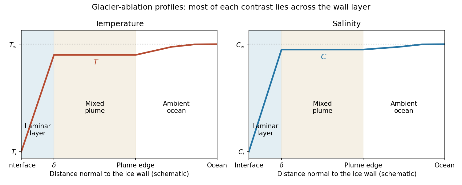
The profiles rise from across the laminar boundary layer to the almost-ambient plume values , then approach across the entraining edge. The sketch uses the linear-gradient approximation implicit in the prescribed diffusive fluxes; it is not an exact normal advection–diffusion profile at large .
For ,The last formula retains both first-order terms and is appropriate near the no-ablation threshold. Salt diffusion keeps the interface saline, and freezing-point depression allows ice dissolution in saline water even when . Latent heat is still needed, but the thermodynamic permission to ablate comes from the depressed liquidus; small does not mean a negligible energy cost.
For , and . Rapid production of fresh melt dilutes the interface, so its temperature approaches the pure-ice melting point. In the usual thermally driven regime and ,This is predominantly thermal melting. More generally the retained large- balance is . For example, gives , which can be large while the driving term is still saline freezing-point depression. Thus the melting/dissolution interpretation must also consider the ocean's temperature relative to , not the compositional Péclet number alone.
Take and , with the liquidus referenced to the pure-water melting point. The solid-liquid segregation coefficient means that newly formed ice contains no salt. A steady sharp front producing only pure ice cannot remove the incoming solute flux. More explicitly, in the liquid the steady solute flux is , whereas in pure solid it is zero. Interfacial salt conservation would require , a contradiction. An equilibrium mushy layer avoids this by carrying concentrated pore liquid down to the eutectic region, where a salt-bearing solid assemblage can form.
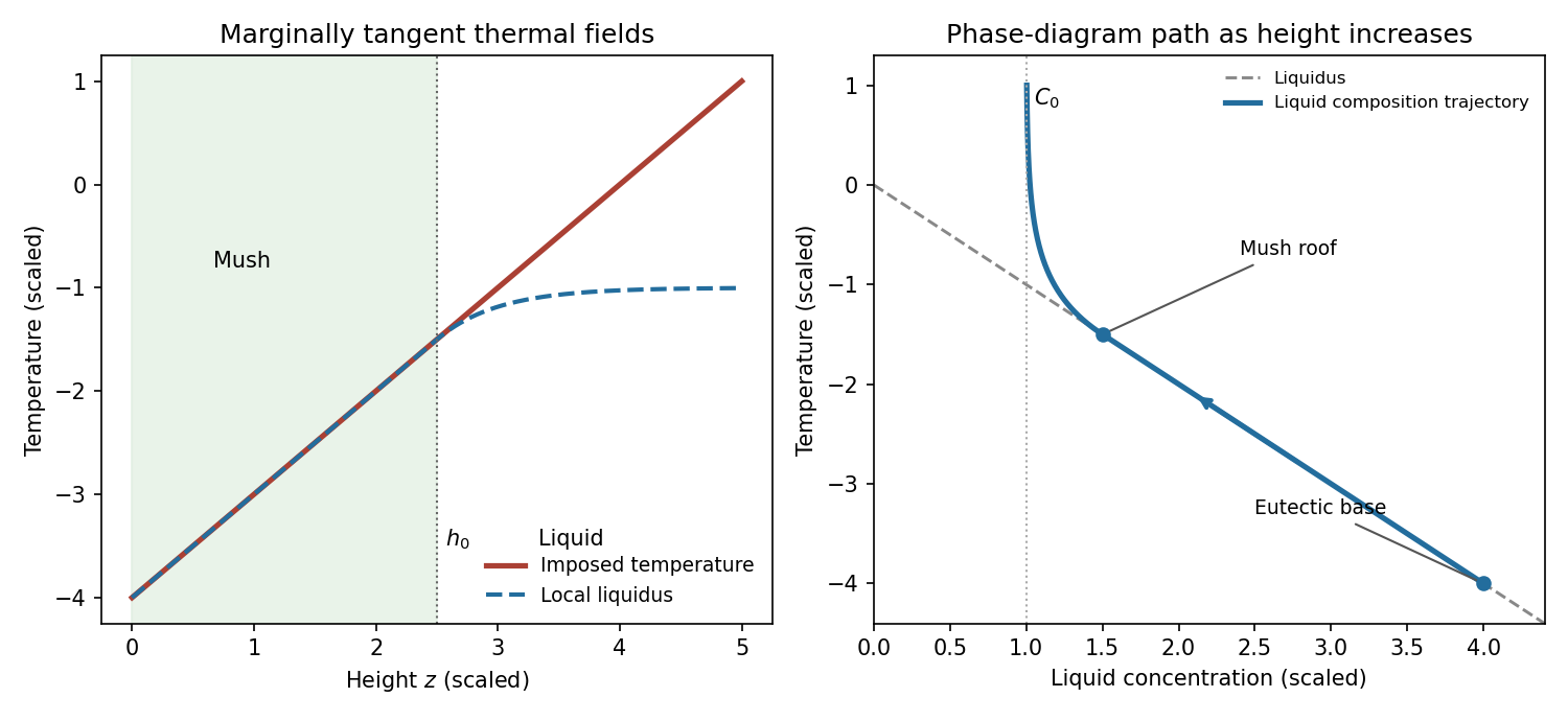
Use equal densities and common downward translation velocity . Write for the liquid fraction; here is the solid fraction. Local liquidus equilibrium in the mush requiresAbove a stationary roof , the liquid advection-diffusion equation is , with solutionThe marginal equilibrium at a mush-liquid boundary condition is , hence . Matching the temperature and liquidus at the roof givesA positive equilibrium mush requires ; otherwise this positive-thickness construction does not apply.
Including solute diffusion in the liquid pore space, the steady solute flux in the mush isThus . Inserting and the value of yieldsThis is the diffusive steadily pulled equilibrium mush. Omitting the diffusive contribution would give a different solid-fraction distribution.
The imposed temperature and local liquidus coincide throughout the mush. In the liquid put . Their difference iswith equality and matching first derivatives at the roof. The inequality follows because the derivative of is . Thus the liquid is not constitutionally supercooled. In the phase diagram, the pore-liquid trajectory follows the liquidus from the eutectic composition to , then curves into the liquid region and approaches as height increases. Pure-ice crystals have composition zero; the trajectory denotes the liquid composition, not the bulk mush composition.


After pulling stops, the imposed temperature keeps the pore-liquid composition fixed wherever the material remains mush. Solute conservation becomesBecause , this reduces toThe method of characteristics uses and . HenceThese are the solute-diffusion characteristics in a fixed-temperature mush; their validity is local to the coexisting solid–liquid region.
For an explicit initial-data solution, define , and , so . A characteristic through has initial footWhile that foot lies in the original mush and no phase boundary has removed the point,This recovers the initial distribution and shows that interior ice fraction increases as salt diffuses upward from colder, more concentrated pore liquid.
If one simply transports the initial zero-solid-fraction level, implies the printed formal lawOn the physical concentration branch , this is , so . It starts moving above immediately.
This formal continuation cannot be the physical mush–liquid roof of a column sealed to salt by the membrane. The no-flux constraint in a fixed-temperature mush is at the membrane. At a smooth zero-fraction equilibrium roof, however, and , giving . Moreover the formal roof has left the membrane-bounded domain. The printed interface law is incompatible with a salt-impermeable membrane when interpreted as the physical roof. Its derivation above is a characteristic extrapolation; it does not enforce the stated boundary condition. If “impermeable” were intended to block bulk flow but allow salt diffusion, a different boundary condition would need to be specified.
The closed-column physical sketch is consequently different. Salt transported upward accumulates below the membrane and produces a liquid brine cap; the cap composition need not lie on the liquidus at every height. Its lower boundary can have a finite jump in solid fraction, so it need not follow the initial zero-fraction characteristic. Near the cold solid base, zero salt supply from below requires the liquid fraction to vanish, and a pure-ice region develops. In the surviving mush, the characteristic formula increases relative to its initial value. An intermediate profile therefore has pure ice at the bottom, a remaining mush with elevated solid fraction, and liquid at the top. The plotted intermediate roof is schematic, not claimed to obey the inconsistent formal law.
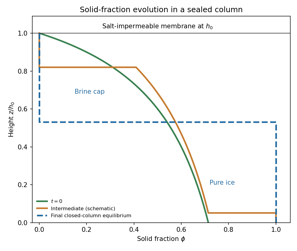
Initial, intermediate and final solid fractions in a salt-sealed column
. Details. 
One can characterize the final state quantitatively if the solid base also admits no salt diffusion, as in the usual pure-solid/no-solid-diffusion closure. In a stationary column, solute flux is constant and is zero at the sealed roof. A finite-width equilibrium mush would have , forcing everywhere in that region; it therefore cannot remain mush. The final state is pure ice for and a uniform-composition liquid cap for . At their boundary,The cap is liquid because above its base. The fixed external thermal field can supply or remove the heat involved; this is a solute-budget determination rather than an isolated enthalpy budget.
The final salt budget of a sealed mush column determines . Initiallysince . Conservation requires . Writing the final cap depth , the equation and its unique positive root areThe initial salt integral is less than , so and ; the resulting remains on the ice–brine branch above the eutectic. If the basal eutectic region is instead allowed to exchange solute with the column, this salt budget must include that flux and the numerical final height is not fixed by the printed data alone. No universal physical follows from the interior characteristic equation without the cap and basal boundary conditions.
Articles by others on the same topic
There are currently no matching articles.