Let . The feasible probability simplex is a nonempty compact convex set, so the extreme value theorem guarantees a minimizer. Its Hessian matrix is diagonal with positive entries , making a strictly convex function. Hence the minimizer is unique.
Use the Lagrange multipliers for the sum constraint and for . The Lagrangian isThe KKT conditions areA strictly positive feasible allocation exists, so the Slater condition holds. These conditions are necessary and sufficient for this convex optimization. At least one coordinate is positive, giving . Put . For a positive coordinate, complementary slackness gives . At a zero coordinate, stationarity gives , or . ThusHere . This logarithmic water filling raises the smaller baseline values to a common level. The scalar left side is a continuous function and strictly increasing above , starts at zero, and tends to infinity, so exactly one solves it. One can find it by interval bisection, or sort the baseline values increasingly and find an index for whichusing . Equality at the next baseline simply gives a zero allocation. Sorting and a running sum implement the water-filling algorithm in time.
The increasing baseline order is . A water-filling algorithm with three active coordinates givesTherefore, in the original coordinate order,The first three shifted coordinates all equal , the fourth remains , and the allocations sum to one. For an explicit KKT certificate take , , and . The strict convexity established above makes this optimum unique.
Write the primal in the form with and . Its dual linear program is with and . Indeed, nonnegative combinations of the primal inequalities give , which is weak duality. The specific dual isThe four dual inequalities correspond, in order, to the four primal variables.
Introduce nonnegative slack variables for the four dual inequalities. The initial simplex dictionary isAt the origin all four basic slacks are positive. Enter : the simplex ratio test compares bounds from and from , so leaves at . Entering initially would tie two limiting bounds and produce degeneracy in linear programming; the chosen pivot avoids this. The new simplex dictionary isOnly has positive objective coefficient. Enter it; the limiting bound is from , rather than from . Thus leaves, givingEvery nonbasic variable has nonpositive objective coefficient, so this feasible simplex basis is optimal. Setting the nonbasic variables to zero yieldsBoth new basic solutions have strictly positive basic coordinates; neither pivot is degenerate.
The first and fourth dual constraints have positive slacks and . Complementary slackness therefore requires . Since , the second and third primal constraints must be equalities:ConsequentlyThe first primal left side is , so the vector is feasible. Its value matches the feasible dual value, giving a linear programming optimality certificate.
For any feasible primal vector, twice the second constraint plus one third of the third givesSince ,The vector is feasible and attains this bound. It is optimal, by this direct inequality proof of weak duality, without assuming the simplex method or a duality theorem. Equality forces and both positively weighted constraints tight, so it also proves uniqueness.
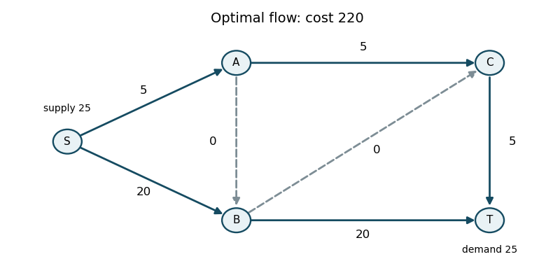
Label the vertices (left), (upper middle), (lower middle), (upper right), (lower right). Use the flow balance convention outgoing minus incoming equals supply. The printed initial flows, in the order , areThey obey all capacity constraints and the flow balances . The four strictly interior edges form a spanning tree. The remaining edges are at a bound: at zero, and at their upper bounds. Thus this is already a feasible network simplex tree basis; no artificial feasibility phase is needed. Its total cost is .
For a tree, choose network dual potentials with and zero network reduced cost on each tree edge. InitiallyThe nonbasic lower-bound edge has network reduced cost . Increase its flow and adjust around the graph cycle , reversing and . The available step is , so leaves at zero. This givesThe tree is now , and the potentials are .
Now is at its upper bound but has network reduced cost , so decreasing it improves cost. Its reverse residual network edge enters along the cycle . The forward edges increase; decrease. The step isThus leaves at its upper bound, andThe new tree has potentials .
The upper-bound edge now has network reduced cost . Enter its reverse direction along , decreasing and and increasing . The step is , so leaves at zero. The resulting flow isThe tree is , with potentials . The nonbasic edges have network reduced costs at its upper bound, at its lower bound, and at its lower bound. All have the correct signs, so there is no improving network simplex pivot. The next part proves these signs certify optimality.
For a minimum-cost flow with bounds , the capacitated flow optimality conditions consist of primal feasibility and network dual potentials whose network reduced costs obeyFor a zero-capacity edge both bounds coincide and no sign restriction is needed; all capacities here are positive. These are the bound form of complementary slackness. To derive necessity directly, construct the residual network: a possible increase has original cost and a possible decrease has reverse cost . An optimal flow cannot admit a negative-cost directed cycle, since a positive step around it preserves flow balance and lowers cost. If there is no such cycle, connect a new source by zero-cost edges to every vertex and let be shortest-path distances. They exist because no negative cycle is reachable. For every residual edge , . Taking makes every residual network reduced cost nonnegative, exactly the displayed sign conditions: both directions exist for an interior edge.
Conversely, for any other feasible flow , equal flow balances giveEach summand is nonnegative at a lower or upper bound, and zero at an interior edge. Hence the sign conditions suffice for optimality as well.
For the final flow, use in the order . All four tree edges have zero network reduced cost, while have costs . More explicitly, every feasible flow satisfiesOur flow attains equality. This gives a direct cost certificate of 220. The strict signs also force , at any optimum; flow balance then fixes all remaining edges, so this flow is unique.
Use the specified construction as a polynomial-time many-one reduction from 3-SAT. There are vertices and edges: one edge per variable pair, three edges per clause triangle in a graph, and three occurrence edges per clause. Any vertex cover must take at least one vertex from every variable pair and at least two from every clause triangle. Therefore every cover has at least vertices.
Given a satisfying Boolean valuation, include the vertex corresponding to the true Boolean literal in each variable pair. In each clause choose a true occurrence and omit its clause vertex, including the other two. Every variable edge and triangle edge is covered. An occurrence edge with an included clause endpoint is covered automatically; the only omitted occurrence vertex is joined to the included true-literal vertex. This is a vertex cover with exactly vertices.
Conversely, a cover of that size must use exactly one vertex in each variable pair and exactly two in each triangle. Declare a variable true precisely when its positive-literal vertex is included. Each clause has one omitted vertex. Its occurrence edge forces the corresponding literal vertex into the cover, so that literal is true. Every clause is therefore satisfied. ThusThe construction and target size are polynomial in the input length. Since 3-SAT is NP-complete, the decision problem is NP-hard. The usual “at most ” version has the same equivalence here because is an unavoidable lower bound. More generally, a cover with fewer than vertices can be padded to exactly . Verifying a proposed cover is polynomial, so the usual vertex-cover decision problem is also in NP and hence NP-complete.
Let the bipartite graph have parts . Add a source , a sink , capacity-one edges for and for , and capacity on each original edge directed . Use the max-flow min-cut theorem: maximum flow value equals minimum cut capacity. Also use Integrality of the Ford-Fulkerson algorithm: integral capacities admit an integral maximum flow, found by integral augmenting paths.
An integral flow selects a matching in a graph, because each left and right vertex carries at most one unit. Conversely every matching gives a unit flow along its selected paths. Hence maximum flow value equals maximum matching cardinality.
A minimum cut has capacity at most , whereas crossing even one original edge would cost . For its source side , no edge of the original graph runs from to . Thereforeis a vertex cover, and its cardinality is exactly the cut capacity. Conversely, given any cover , use . No original edge crosses this cut, because both its endpoints would otherwise be outside the cover; its capacity is . Thus minimum cut capacity equals minimum cover size, proving König's theorem for bipartite matching:For the algorithm, repeatedly find augmenting paths in the residual network, then take to be the vertices reachable from . Each integral augmentation increases flow by at least one; the total value is at most . Each reachability search takes time, so this procedure takes time. The network uses only polynomially many edges and integer capacities, yielding the requested polynomial-time algorithm and an explicit cover.
Let be the row payoff matrix and . For in the probability simplex , write and define the symmetric Nash gain mapThe map is a continuous function, has nonnegative coordinates, and sums to one. The Brouwer fixed-point theorem states that every continuous self-map of a nonempty finite-dimensional compact convex set has a fixed point. Apply it to , and let .
Set . The fixed-point equation gives . If , every positive has strictly positive gain, so . Buta contradiction. Thus and every pure payoff is at most . Since their -weighted average equals , every supported action attains that maximum. Consequently is a best response to itself.
The column player's payoff vector against is , so exactly the same inequalities establish its best response. ThereforeThis supplies the whole fixed-point construction and fixed-point-to-equilibrium argument, rather than assuming Nash's theorem as a black box.
The matrices obey , so both players' pure best response vectors have the form against opponent mixture . Against pure actions , the unique best responses are respectively . This three-cycle has no mutual best-response pair, so there is no pure Nash equilibrium.
In a game satisfying nondegeneracy of a bimatrix game, the two equilibrium strategy supports have equal cardinality: each support consists of best responses to the other strategy, so each size is at most the other. If both supports have size three, must have all coordinates equal. The first-minus-second and second-minus-third equations implyThis has no fully positive simplex solution. Thus both supports have size two.
For full support enumeration for a bimatrix game, denote the three possible supports by . On equal supports and , indifference requires respectively probabilities and , so those pairs fail. Equal support gives , whose omitted-action payoff is . The cross pair yieldswith and . Thus the supported actions are best responses. Its reversed pair is also an equilibrium. The remaining unordered cross pairs fail: for the necessary gives , so the opponent has a profitable action outside its support. For , the necessary opponent mixture on is , which is infeasible. Reversing either failed pair cannot rescue it.
Hence all three equilibria areTheir payoffs are respectively , and . The support-size argument and exhaustion above rule out every other equilibrium.
The equilibrium oddness theorem gives a finite odd number of Nash equilibria in a finite nondegenerate bimatrix game. One way to see the parity is through the endpoint argument underlying the Lemke-Howson algorithm. Add sufficiently large constants to each payoff matrix so all entries are positive; this does not change best responses. Form the bounded convex polytopesLabel an facet by row label and a tight facet by column label ; in , label a tight facet by and by . A completely labelled vertex of a polytope pair has either both vectors zero, or both nonzero and normalizes to a Nash equilibrium. In the latter case the labels express exactly the equilibrium best-response and zero-probability conditions. Nondegeneracy makes each vertex of a polytope have exactly distinct incident labels and each equilibrium correspond to one such pair.
Fix a label to drop and retain all pairs carrying every other label. Include the product-convex polytope edges that retain those labels. At a completely labelled pair there is one possible outgoing edge, obtained by dropping the fixed label. At any other retained vertex of a polytope, that label is missing and one other label is duplicated; dropping either copy gives the two incident edges. Thus this finite graph consists of paths and cycles, with its endpoints precisely the completely labelled pairs. A finite graph has an even number of degree-one vertices. Since one endpoint is the artificial zero pair, the number of genuine equilibrium endpoints is odd. This proves the required equilibrium oddness theorem and finiteness, without claiming that every equilibrium is reached from the zero pair on the same path.
For a symmetric bimatrix game, swapping players maps to . Every nonsymmetric equilibrium lies in a distinct two-element pair; the fixed points of this involution are exactly the symmetric equilibria. Removing even-sized pairs from an odd total leaves an odd number of symmetric equilibria. In the present game, two equilibria form the swapped pair and the remaining one is with . There is exactly one symmetric equilibrium, as required.
Use the usual essential two-person Nash bargaining problem: is a compact convex set, is the disagreement point, and some satisfies for both players. The Nash bargaining solution isThe positive maximum exists by compactness and essentiality. On positive gains, maximizing this Nash product is equivalent to maximizing , a strictly concave function. Convexity then gives a unique maximizer. The essentiality and compactness hypotheses matter: for example, with and , the product is zero everywhere and its argmax alone is not a single-valued definition.
The rule satisfies all four axioms. Pareto efficiency: a feasible vector dominating the chosen vector with at least one strict improvement would increase its positive Nash product. Bargaining symmetry: if the problem is unchanged by swapping players, uniqueness makes the answer unchanged, so the two payoffs agree. Positive affine invariance in bargaining: for with , gains transform to and the product is multiplied by the positive constant , preserving its maximizer. Bargaining independence of irrelevant alternatives: if is another admissible feasible set containing the chosen vector and the same disagreement point, that vector remains the unique product maximizer over .
To prove characterization, let be any feasible single-valued rule satisfying these axioms, and let . Normalize payoffs by the positive affine transformationThe transformed set has disagreement point zero and product maximizer . For any , convexity puts in ; for sufficiently small both gains remain positive. The one-sided derivative of the product at its maximum is therefore nonpositive:Thus . By compactness choose so every coordinate of every is at least . The supporting triangle for Nash bargaining isIt contains , is compact, convex, symmetric and essential, and contains disagreement zero. Symmetry forces onto the diagonal; Pareto efficiency then forces it to be . Since , bargaining independence of irrelevant alternatives gives . Undoing the normalization by positive affine invariance in bargaining gives . Hence the four axioms uniquely characterize the Nash bargaining solution on this domain.
A security level payoff maximizes what a player guarantees against the opponent. Let be the row player's probability of the first action. Its guaranteed payoff isThe decreasing and increasing terms cross at , attaining ; moving either way lowers the smaller term. For the column player, any mixture has zero payoff against the first row, while its second-row payoff is nonnegative. Therefore andThe feasible set is the convex hull of the four joint pure-action payoff vectors. Its upper Pareto frontier connects to to . Write the row payoff as and column payoff as . On the first Pareto frontier segment, for . The Nash product isa concave quadratic with derivative , maximized at , , giving product . On the portion of the other Pareto frontier segment satisfying bargaining individual rationality, and . Its product derivative is positive throughout, so its largest product is at , smaller than . All dominated points can be discarded by Pareto efficiency. ConsequentlyThis payoff is implemented by a correlated payoff lottery choosing the payoff with probability and with probability . The convex hull permits such lotteries over joint outcomes; it is not restricted to independent mixed strategies.
Transposing the second player's matrix leaves the row player's security level payoff at . The column player's second action now yields payoffs and , while its first yields zero for either row. Its security level payoff is therefore , guaranteed by the second action; against the first row no mixture can guarantee more. Thus .
The relevant upper Pareto frontier joins the payoff vectors and , so . On the segment satisfying bargaining individual rationality , the Nash product becomesIts derivative is and its second derivative is . HenceThe implementing correlated payoff lottery chooses with probability and with probability . Both players' gains are strictly positive: and . The new disagreement point must be recomputed after transposition; reusing the previous column security payoff would solve a different Nash bargaining problem.
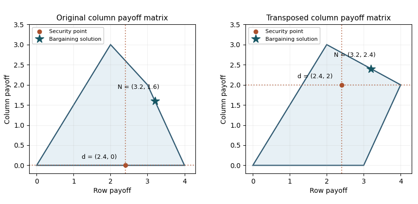
Feasible payoff polygons, security points and Nash bargaining solutions before and after transposing the column payoff matrix
. Articles by others on the same topic
There are currently no matching articles.