Past exam of the mathematics course of the University of Cambridge / 2015 / iii / Paper 40 (Advanced Financial Models)

Put ${\mathcal{L}}_{r}V(s)=\frac{1}{2}{\sigma }^2{s}^2{V}^{\prime \prime }(s)+rs{V}^{\prime }(s)$ and define the nonnegative reserve rate $a(s)=rV(s)-{\mathcal{L}}_{r}V(s)$. The obstacle problem gives $V\ge g$ and $a\ge 0$. The American-option superhedge with a funded reserve invests the local surplus in the bond rather than consuming it.

For initial wealth $x\ge V(S_0)$, setand choose the stock and bond holdingsThus $D_t\ge 0$ and $F_t\ge V(S_t)\ge g(S_t)$, pathwise at every time. The Itô formula under the original drift givesAdding these equations yieldsThis is a self-financing strategy, and its nonnegative wealth makes it an admissible trading strategy. Continuity of the stock and local regularity of $V$ ensure local integrability of the holdings. The construction does not require $\mu =r$.

For a classical solution, the usual Itô formula applies directly. The smooth fit solution below is $C^1$ and piecewise $C^2$, with locally absolutely continuous first derivative. The generalized Itô formula applies with its almost-everywhere second derivative; the absence of a derivative jump means no boundary local time of a semimartingale term. This is the usual regularity interpretation of the perpetual American option obstacle equation.

Write $\alpha =2r/{\sigma }^2\in (0,1)$. In a continuation interval, the Euler differential equation has power solutions $s$ and $s^{-\alpha }$: substitution of $s^{\beta }$ gives $(\beta -1)(\beta +\alpha )=0$. A decreasing bounded value uses the second solution.

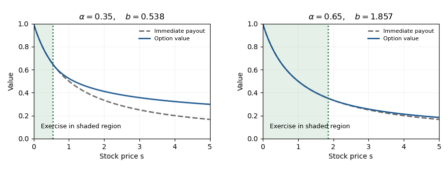
Let $b$ be the exercise boundary. Value matching and smooth fit require $A{b}^{-\alpha }=(1+b{)}^{-1}$ and $-\alpha A{b}^{-\alpha -1}=-(1+b{)}^{-2}$. Dividing gives $b/(1+b)=\alpha$. ConsequentlyThis is a perpetual reciprocal-payoff American option.

To verify the obstacle inequality, observe that $s^{\alpha }/(1+s)$ increases up to $b$ and decreases afterwards, because its logarithmic derivative is $\alpha /s-1/(1+s)$. Therefore $V(s)\ge (1+s{)}^{-1}$ for $s>b$. In the continuation region $({\mathcal{L}}_r-r)V=0$. In the exercise region,The quadratic is convex. At the two endpoints of $[0,b]$ it equals $-\alpha /2$ and $-\alpha /[2(1-\alpha )]$, respectively, so it is negative throughout that interval. Thus the obstacle problem is satisfied on both regions, with value matching and smooth fit at $b$. The second derivative has a jump at $b$; the equation is understood piecewise and in the generalized Itô sense described in part (a).

For optimality, use the Risk-neutral measure for the Black-Scholes model, under which $d{S}_t=r{S}_{t}dt+\sigma S_{t}d{W}_t^{\mathbb{Q}}$. The Itô formula makes $e^{-rt}V(S_t)$ a nonnegative supermartingale, so every exercise time $\tau$ satisfiesBefore hitting the exercise region, its drift vanishes. Since $0\le V\le 1$, the stopped process is a bounded martingale. Apply the optional sampling theorem at ${\tau }_{\ast }\wedge T$ and let $T\to \infty$. The contribution from $\{{\tau }_{\ast }>T\}$ is at most $e^{-rT}$, while the boundary value equals the payoff. Hence equality holds forIf $S_0\le b$, exercise immediately; otherwise wait for the first down-crossing. If that time is infinite, the discounted payout is zero. This proves both the value and the optimal stopping policy, and part (a) supplies its superhedge.

Interpret positivity of $Y$ as strict positivity almost surely. Suppose the stated bounded positive pricing variable exists. For a vector $H$ satisfying the two sign restrictions,A nonnegative random variable with zero expectation vanishes almost surely. Since $Y>0$, this gives $H\cdot P=0$ almost surely and $H\cdot p=0$. The supplied nondegeneracy condition now yields $\boxed{H=0}$. This proves the direction from a one-period martingale deflator to the separating-portfolio condition; no asset-pricing theorem has been invoked.

A direct exponential minimization construction of a bounded pricing kernel proves the reverse implication without using a course theorem. ConsiderBoundedness of $P$ makes $F$ finite, continuous, and differentiable. On every bounded set of $h$, the exponential and its derivatives have deterministic bounds, so differentiation under expectation is justified.

We first prove coercivity: $F(h)\to \infty$ as $|h|\to \infty$. Otherwise there would be a sequence $h_j$ with $|h_j|\to \infty$ along which $F(h_j)$ stays bounded above. Pass to a subsequence with $h_j/|h_j|\to u$, $|u|=1$. There are two cases.

If $\mathbb{P}(u\cdot P<0)>0$, choose $a>0$ with $\delta =\mathbb{P}(u\cdot P\le -a)>0$. The bound on $P$ gives $h_j\cdot P\le -a|h_j|/2$ on this event for all large $j$. ThereforeIf instead $u\cdot P\ge 0$ almost surely, the portfolio condition forces $u\cdot p>0$, since $u\ne 0$. Hence $h_j\cdot p\to \infty$, and the nonnegative exponential term again forces $F(h_j)\to \infty$. Both cases contradict the chosen sequence.

A minimizing sequence is consequently bounded. It has a convergent subsequence, and continuity of $F$ gives a global minimizer $h_{\ast }$. At a minimizer each directional derivative vanishes, soThusIf $|P|\le L$, then $e^{-|h_{\ast }|L}\le Y\le e^{|h_{\ast }|L}$: the constructed pricing kernel is bounded and even bounded away from zero. The compactness, coercivity, and differentiation arguments above supply the needed proof rather than appealing to the fundamental theorem of asset pricing.

Use the positive variable $Y$ from part (a). Since $0\le (S-B{)}^{+}\le S$ and $(S-B{)}^{+}\ge S-B$,Combining these inequalities gives the one-period call price boundsFor the strict assertion, both $\{S>B\}$ and $\{S<B\}$ have positive probability. Positivity of $Y$ givesIf $s-b\ge 0$, the second inequality is the required strict bound; if $s-b<0$, the first is. Hence $\boxed{c>(s-b{)}^{+}}$. The weighted expectations are finite because $P$ and $Y$ are bounded.

A complete market permits claim replication for every finite maturity and every bounded claim measurable at that maturity: there are an initial capital and a predictable self-financing portfolio whose terminal wealth equals the claim almost surely. In a finite-state market this is equivalent to replicating every terminal payoff, since all such payoffs are bounded. Trading is allowed dynamically in the existing $n$ assets; adding a new security is not part of the definition.

We prove the stronger finite branching bound in a complete market: modulo null sets, ${\mathcal{F}}_t$ is generated by at most $n^t$ atoms. Here an atom is a positive-probability event which cannot be split into two positive-probability measurable pieces.

At time zero there is one atom because ${\mathcal{F}}_0$ is trivial. Suppose ${\mathcal{F}}_{t-1}$ has at most $n^{t-1}$ atoms, and fix one such atom $A$. Any predictable process holdings over $(t-1,t]$ are constant on $A$, so the restriction to $A$ of every time-$t$ replicable payoff lies ina vector space of dimension of a vector space at most $n$. If $A$ contained $n+1$ disjoint positive-probability ${\mathcal{F}}_t$ events, their indicators would have linear independence on $A$. Market completeness would replicate each indicator, contradicting that dimension bound.

For clarity, the absence of $n+1$ disjoint positive pieces implies that $A$ is a union of at most $n$ atoms: start with $A$ and repeatedly split any non-atom into two positive pieces. Each split increases the count by one. The process must stop before the count exceeds $n$, and at termination every piece is an atom. Thus each time-$(t-1)$ atom has at most $n$ successors. Induction gives at most $n^t$ atoms at time $t$.

Each disjoint positive-probability ${\mathcal{F}}_t$ event contains at least one distinct atom. ThereforeThe argument includes $t=0$ and uses the ability to replicate the indicator claims at every intermediate maturity.

Use the conditional second-moment matrix $V_t=\mathbb{E}[P_t{P}_t^{\top }\mid {\mathcal{F}}_{t-1}]$ from the PDF. By part (b), the filtration is finite-state at every finite time. On a time-$(t-1)$ atom let $p_1,\dots ,p_m$ be the successor price vectors and $q_1,\dots ,q_m>0$ their conditional probabilities. Then $m\le n$ andPositive definiteness gives rank $n$, so $m\ge n$. Hence $m=n$, and the $n$ successor vectors have linear independence.

We use the finite-horizon fundamental theorem of asset pricing in deflator form: an arbitrage-free finite market admits a strictly positive adapted process $D$, with $D_0=1$, such that $DP$ is a martingale. Equivalently, on every step,Fix a finite horizon containing the step in question. On the parent atom, write $d_i=D_t/D_{t-1}>0$ on successor $i$ and $p_0=P_{t-1}$. ThenThe proposed values $z_i=p_i^{\top }{V}^{-1}{p}_0$ satisfy precisely the same equation:Because the $p_i$ have linear independence and the $q_i$ are positive, this linear system has a unique solution. Thus $z_i=d_i>0$, provingThis is the positive regression deflator in a complete finite market. It also proves the suggested conclusion: with $Y_0=1$ and $Y_t={\prod }_{u=1}^t{Z}_u$,Hence $Y$ is a strictly positive martingale deflator. Finite-state structure makes these expectations integrable on each finite horizon. Positive definiteness alone would not ensure positivity of the regression factor; market completeness and the positive deflator are essential.

For $S_0>0$, the stochastic exponential solution stays strictly positive. Put $U_t=\sqrt{S_t}$. The Itô formula givesThus $U$ is a nonnegative local supermartingale. To justify the true supermartingale property, stop where $U$ or its stochastic integral exceeds successive bounds. The stopped Itô formula gives $\mathbb{E}[U_{T\wedge {\tau }_m}\mid {\mathcal{F}}_t]\le U_{t\wedge {\tau }_m}$ for $T\ge t$. The conditional Fatou lemma and ${\tau }_m\uparrow \infty$ yieldIn particular $\mathbb{E}{U}_T\le U_0<\infty$. The case $S_0=0$ is the identically zero process. This is the square-root stock supermartingale.

The coefficient is $\boxed{k=1/8}$, but independence alone does not make the printed right-hand side ${\mathcal{F}}_t$-measurable. The future variance integral need not be known at time $t$. This is a genuine missing information assumption in the PDF.

The Itô formula or explicit stochastic exponential givesIf the volatility path is fixed at time zero and independent of $W$, conditioning on that path makes the first factor an exponential of a centered Gaussian variable with the compensating half-variance, so its conditional expectation is one. More generally, this conditioning works when enlarging the filtration by the entire independent volatility path preserves the Brownian property. For the usual joint filtration of Brownian history and independent volatility history, the valid conditional square-root price under independent volatility isWhen the integral is already ${\mathcal{F}}_t$-measurable, the outer conditional expectation can be removed, giving the intended printed formula. In particular this holds for deterministic volatility or an independent path disclosed initially.

For a counterexample to the unqualified printed assertion, take an independent fair Bernoulli variable $A\in \{0,1\}$, disclose it at time $1$, and letWith the filtration generated by the Brownian history and this disclosure, $W$ is Brownian and $\sigma$ is bounded, continuous, adapted, and independent of $W$. At $t=0,T=2$, the variance integral is $A/3$, while ${\mathcal{F}}_0$ is trivial. Direct Gaussian conditioning givesa constant. The proposed factor $e^{-A/24}$ is random, so cannot equal that conditional expectation. The formula requires knowledge of future integrated variance; independence by itself is insufficient.

This part's conditional-expectation representation is its own hypothesis; it does not need the incorrect unrestricted claim in part (b). Fix $T$, and writeThe assumed representation makes $M(T)$ a martingale. The stochastic Fubini theorem givesApply the Itô formula to $e^{-I}$ and use the equation for $U$ from part (a), including the cross-variation. The result isUniqueness of the continuous semimartingale decomposition makes the drift vanish. Initially this is a $dtd\mathbb{P}$ statement; the assumed continuity in time and maturity extends it to the continuous versions simultaneously. Let $T\downarrow t$ to obtainSubstitute back and differentiate the maturity integrals using their continuous integrands:This is the forward drift restriction for square-root stock claims. The $-{\sigma }_t/2$ term comes from the product cross-variation and must be retained. For the uninformative zero-stock case, the representation does not identify $f$; as usual a positive initial stock price is understood.

Use a telescoping replication of a stock-price sum. Hold $T-t+1$ shares during interval $(t-1,t]$; at time $t$, sell one share and keep its proceeds in the bond. Start with $T$ shares and no cash, costing $T{S}_0$.

After the time-$t$ rebalance, the stock holdings are $T-t$ and the cash holdings are ${\sum }_{u=1}^t{S}_u$, so wealth isThe sale of one share exactly funds the cash increase, making the strategy self-financing. Equivalently,At time $T$ there are no remaining shares, and the cash equals the claim. All stock positions over trading intervals are predictable.

For every integer $m\in \{0,\dots ,N\}$,Thus the static replication on a finite terminal support consists of one share and two calls of every listed strike, held to maturity:The strike-$N$ call contributes zero at maturity but is harmless in this identity. The portfolio costs $S_0+2{\sum }_{K=1}^N{C}_0(K)$. No distributional assumption on the stock is needed beyond its stated terminal support.

The pathwise identity $(S_t-S_{t-1}{)}^2=S_t^2-S_{t-1}^2-2S_{t-1}(S_t-S_{t-1})$ telescopes toThis is the discrete realized-variance replication identity. Replicate $S_T^2$ using part (b). Add a self-financing portfolio with initial wealth $-S_0^2$ and stock holdings $-2S_{t-1}$ during $(t-1,t]$.

To give the cash positions explicitly, letThe added portfolio holds $G_{t-1}+2S_{t-1}^2$ units of the bond over that interval. Its starting value is $G_{t-1}$ and its change is exactly $-2S_{t-1}(S_t-S_{t-1})$. The combined holdings are thereforeThe terminal value equals the squared-increment sum by the telescoping identity. Its initial cost isThe dynamic stock hedge uses only prices known before each interval, while the calls remain static.

Normalize $B_0=1$ and put ${\tilde{S}}_t=e^{-rt}{S}_t$. Its dynamics are $d{\tilde{S}}_t={\tilde{S}}_t\sigma (t,S_t)d{W}_t$. Bounded volatility makes this stochastic exponential a true martingale on each finite horizon, by the Novikov condition. It also gives a finite second moment: stopping the Itô formula for $S^2$ and applying the Gronwall inequality yields $\mathbb{E}{S}_T^2\le S_0^2{e}^{(2r+L^2)T}$ when $\sigma \le L$.

The discounted payoff $\xi =e^{-rT}(S_T-K{)}^{+}$ is thus square-integrable. Define the nonnegative martingaleThe Brownian martingale representation theorem says that every square-integrable martingale in the Brownian filtration has a representation $M_t=M_0+{\int }_0^t{h}_{u}d{W}_u$ with predictable $h$ and $\mathbb{E}{\int }_0^T{h}_u^{2}du<\infty$. Since $\tilde{S}>0$ and $\sigma >0$, chooseThen discounted gains satisfy $d{M}_t={\pi }_{t}d{\tilde{S}}_t$. Consequently $X_t=B_t{M}_t={\varphi }_t{B}_t+{\pi }_t{S}_t$ is self-financing, nonnegative, and hence an admissible trading strategy. At maturity $X_T=(S_T-K{)}^{+}$, proving claim replication at cost $C(T,K)$.

For minimality, discounted wealth of any admissible self-financing portfolio is a local martingale bounded below, hence a supermartingale by localization and the conditional Fatou lemma. Thus any such replication with initial wealth $x$ obeysTogether with the constructed portfolio, this provesThis is Brownian representation replication in a local volatility market. The given drift $r$ means that the original probability measure already serves as the risk-neutral measure.

Differentiating the European call option price in strike gives, for $T>0$,The strike derivative uses dominated convergence; the second uses the continuous density. Also,Differentiate the supplied time-integral identity and the discount factor. Continuity of the density supplies the diffusion-term derivative. For the tail first moment, continuity in time follows from continuous stock paths, locally uniformly bounded second moments, and the absence of an atom at $K$. ThereforeHence the Dupire equation isIts initial condition is $C(0,K)=(S_0-K{)}^{+}$; natural strike boundaries are $C(T,0)=S_0$ and $C(T,K)\to 0$ as $K\to \infty$. These are consistent with the discounted stock martingale and integrable tails. Where $C_{KK}>0$, the same identity gives local volatility recovery from call prices:The equation evolves in maturity and strike, unlike the backward option-value equation in calendar time and spot.

The Brownian martingale representation theorem argument in part (a) also replicates the bounded put payoff. The discounted stock is a true martingale, so the elementary terminal payoff identity yields put-call paritySet $H(T,K)=-S_0+K{e}^{-rT}$. Then $H_T=-rK{e}^{-rT}$, $H_K=e^{-rT}$, and $H_{KK}=0$. ThusLinearity of the Dupire equation and $P=C+H$ giveThe initial payoff is $P(0,K)=(K-S_0{)}^{+}$, and $P(T,0)=0$. Therefore calls and puts obey the same maturity-strike differential equation, with their respective initial and boundary data.