Use the nonnegative sign convention for the Laplace-Beltrami operator; the ambient Laplacian has the same sign convention. Changing both signs changes the signs of the eigenvalues below. Let be an orthonormal basis of , and let be the unit-speed geodesic with and . The geodesic Hessian formula givesIndeed, the second derivative along a geodesic is , because its covariant acceleration is zero. Taking the trace of the Hessian matrix in this orthonormal basis gives the displayed Laplace-Beltrami operator.
For the sphere, put , where , and write for a smooth ambient function. The Euclidean metric becomes and its volume form is . The coordinate formula for the Laplace-Beltrami operator therefore gives the polar-coordinate Laplacian identityFor , restriction to yieldsThis relation also has a direct geodesic proof. At a point , complete an orthonormal basis of the tangent space by the radial vector . Each great-circle geodesic satisfies . The chain rule gives . Summing and comparing with the ambient trace gives precisely the radial correction above.
Let be the space of homogeneous polynomials of degree on , and let be its subspace of harmonic polynomials. For , homogeneity gives . Substituting in the polar-coordinate Laplacian identity proves that its restriction is a spherical harmonic withRestriction is injective on : if , homogeneity makes zero away from the origin, hence everywhere.
To count and exhaust these eigenfunctions, use the harmonic decomposition of homogeneous polynomialsHere is an algebraic proof rather than an assumption about the spectrum. On polynomials put the Fischer inner product . Multiplication by is adjoint to , so multiplication by is adjoint to . In finite-dimensional inner product spaces, the orthogonal complement of the image of multiplication by is . This proves the decomposition. Multiplication by is injective, sowhere the second term is zero for .
Iterating the harmonic decomposition of homogeneous polynomials and restricting to expresses every polynomial restriction as a finite sum of spherical harmonics. Polynomial restrictions contain constants and separate points of the sphere, so the Stone-Weierstrass theorem makes them uniformly dense in the continuous functions, and hence dense in . The Laplace-Beltrami operator is self-adjoint, and eigenfunctions with different eigenvalues are orthogonal. If a smooth eigenfunction had an eigenvalue not in the list, it would be orthogonal to a dense subspace and would vanish. If it had a listed eigenvalue, subtracting its orthogonal projection onto the corresponding finite-dimensional gives the same contradiction. Thus, for , the spectrum of the Laplacian on a sphere isIn particular, the zero eigenvalue has multiplicity one; on each positive eigenvalue has multiplicity two; on the multiplicity is .
A flat torus is the quotient , where is a full-rank Euclidean lattice, with the Riemannian metric induced from the Euclidean metric. Translation by a lattice vector is a Riemannian isometry, so this metric is well defined and has zero curvature. Its volume is the covolume of .
The dual lattice is . For , the function descends to the flat torus, and direct differentiation givesConversely, write and . Ordinary Fourier series on have frequencies , corresponding to . After normalization they form a complete orthonormal basis in , and the Fourier coefficients of a smooth function decay rapidly. Applying the Laplace-Beltrami operator term by term shows that a smooth eigenfunction with eigenvalue has nonzero coefficients only where . Thus the spectrum of a flat torus isThe formula counts multiplicity over either the real or complex numbers: the two frequencies give the real sine and cosine functions.
For the rigidity assertion in dimension two, it suffices to reconstruct a rank-two Euclidean lattice from its vector-length multiset. The multiset first determines its covolume . Indeed, a bounded fundamental parallelogram, and comparison of the cells meeting a disk with slightly larger and smaller disks, give the lattice-point asymptotics by fundamental cellsThe spectrum determines , including multiplicities, so it determines .
Let be the smallest nonzero vector length, and choose with . This vector is primitive: with would contradict minimality. From the length multiset subtract the two vectors at every positive length , for . The shortest remaining length is exactly the length of a shortest vector . This subtraction is legitimate even if several directions have length : it subtracts just two copies, and then . It also proves that is independent of our choice of shortest direction. Replace by to arrangeThe replacement stays outside and cannot be shorter than , so a reduced choice still has length .
The shortest-independent-vector basis lemma says that are a basis of . To prove it, choose coordinates with . Because is primitive, ; let be the smallest positive vertical coordinate in . Write , with after changing its sign. If , a vector of vertical coordinate , reduced horizontally modulo , hasThis contradicts the definition of , since . Hence and generate .
The Gram matrix of this basis is , with , and its determinant is . ThereforeChanging the sign of one basis vector allows . The numbers , all audible from the spectrum, consequently determine the Gram matrix, and hence , up to an orthogonal transformation. Taking dual lattices gives the same conclusion for . Isospectral flat two-dimensional tori are isometric. The argument uses the special basis property of rank-two Euclidean lattices, so it does not claim higher-dimensional rigidity.
A useful precise form of the transplantation theorem is as follows. Take congruent copies of a Euclidean tile with labelled flat faces. For each face colour , encode the gluings by a symmetric signed permutation matrix : a glued pair gives off-diagonal entries in the two corresponding positions; an unglued face gives a diagonal entry for a Dirichlet boundary condition, or for a Neumann boundary condition. Corresponding face identifications must use the same maps in the tile coordinates. Suppose two assemblies have matrices and and there is an invertible matrix withThen, for every eigenvalue , is an isomorphism between their Laplacian eigenfunction spaces. The two assemblies are isospectral, including multiplicities.
To see why, pull every tile restriction back to the same Euclidean tile. A boundary value vector and an outward normal derivative vector satisfyAt an internal face these are continuity of the function and equality of oppositely directed derivatives. At a diagonal they impose ; at a diagonal they impose . The intertwining identities preserve both equations, and the Euclidean Laplacian commutes with constant linear combinations of tile functions. The resulting piecewise function is a weak eigenfunction, with the prescribed boundary conditions, and interior elliptic regularity makes it smooth wherever the assembled manifold is smooth. At polygonal corners one uses the usual weak domain of the Dirichlet Laplacian or Neumann Laplacian, rather than assuming smoothness through a corner. The inverse matrix gives the inverse transplantation.
Here is a completely specified propeller pair. Label the seven triangles , with central triangle , and colour the three sides . In the left and right assemblies the internal-edge pairings areEvery pair means reflection of one triangle across the indicated side; the other faces are external boundary. Each assembly has a central triangle and three two-triangle arms. These are the propeller domains. The drawing uses one acute scalene triangle, and each colour always denotes the side opposite the same marked vertex of the starting triangle.
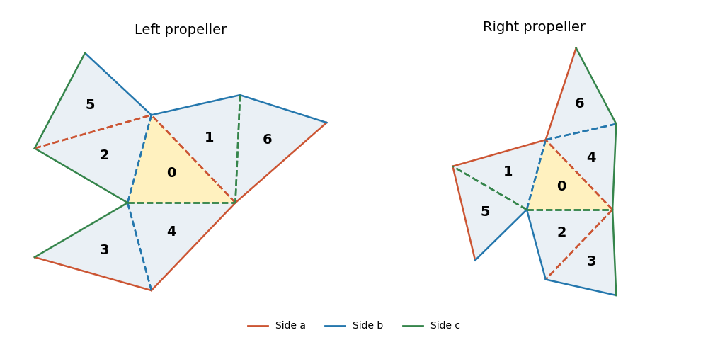
Two seven-triangle propeller domains with the same side-colour gluing rules and different arm orientations
. Details. Let be the ordinary permutation matrices obtained by adding fixed points to the pairings. The following matrix supplies the Neumann boundary condition transplantation:There is a short way to construct and check it. Start with the support in row , and require the support in row to be applied to the support in row . Traversing the six edges of the right-hand tree gives exactly the displayed rows; checking the remaining fixed-point relations verifies for all three colours. Every row has three ones and every two different rows meet in exactly one column, soThe right-hand side has eigenvalues once and six times, proving is invertible, with . Its incidence pattern is that of the Fano plane, which explains the uniform intersections.
For the Dirichlet boundary condition, put . In both assemblies this gives opposite signs to adjacent triangles. Thus their signed face matrices are and : the off-diagonal gluing entries are positive and the unpaired diagonal entries are negative. The matrixthen satisfies and is invertible. The transplantation theorem proves equality of the Dirichlet Laplacian spectra; proves equality of the Neumann Laplacian spectra as well.
Finally vary the three labelled side lengths of the initial triangle in an open region of strict triangle inequalities, with an acute scalene shape sufficiently close to an equilateral triangle. Reflection constructs both domains continuously from these three independent real parameters. At the equilateral configuration the tiles have disjoint interiors. Choose a sufficiently small neighbourhood of that configuration with every triangle angle in . At each central vertex exactly four tile angles meet, forming a sector of angle , while nonincident pieces stay separated. Thus there is an open three-dimensional parameter region in which both assemblies are embedded planar domains.
For a scalene triangle in this region, the three central vertices are exactly the three reflex boundary vertices: their interior angles are , while the other boundary vertices have angles or . Hence a planar isometry of the domains must map the central triangle onto the central triangle. Put those two central triangles in the same position. Their unequal side lengths force any such isometry to fix the central triangle pointwise. Yet the first arm across, for example, side attaches its outer triangle across colour in , and across colour in . These occupy different positions, so the identity does not identify the domains. An intrinsic Riemannian isometry between connected planar domains also restricts locally to a rigid Euclidean motion and hence is one globally. The two propellers are nonisometric throughout this open three-parameter family. Scaling is included as one of the parameters; modulo scaling the family has two parameters.
Let be the orientation-preserving hyperbolic triangle group, acting on the hyperbolic plane with presentationIts quotient is a topological sphere with three cone points of order seven. Define the surjective group homomorphismThe stated order conditions make this well defined, and the generation hypothesis makes it surjective. Set . Every finite-order element of a hyperbolic triangle group is conjugate to a power of a cone-point generator. None of its nontrivial such powers lies in , since all three images have order seven. Therefore is torsion free, and is a closed oriented hyperbolic surface carrying an isometric action of .
The orbifold Euler characteristic of the base isThe covering degree is , so and has genus . The subgroups have order . Point stabilizers for the action are trivial or cyclic of order seven. Since seven does not divide , each acts freely. Thusare smooth closed hyperbolic surfaces, andEquivalently, each is a seven-sheeted orbifold cover of the base with three branch values, and the Riemann-Hurwitz formula gives the same genus.
Gassmann equivalence means that meet each conjugacy class of in the same number of elements. To prove isospectrality directly, let be a Laplacian eigenfunction space on , viewed as a representation of . Pullback identifies with its -invariant subspace. Averaging over is the projection onto this subspace, and henceThe character of a representation in this sum is constant on conjugacy classes. The sums are equal by Gassmann equivalence, so the eigenvalues and their multiplicities agree. This is the mechanism of the Sunada theorem. The constructed genus-three hyperbolic surfaces are isospectral.
Nonconjugacy of in does not prove nonisometry. For example, an isometry of outside the given subgroup might conjugate to and descend to an isometry of the quotients. More generally, an isometry between the quotients lifts to an isometry of conjugating the two groups ; there is no requirement that this lift come from an element of . Additional symmetries of the three-cone-point construction are a possible source of this coincidence.
One can prevent this by modifying the common metric, while keeping the action isometric. Here is a geometric way to make that step precise. On the regular part of the base orbifold , choose a sufficiently small smooth conformal rescaling of a Riemannian metric of its metric whose local geometry distinguishes base points and local directions. One may use a generic smooth conformal factor with separate curvature features on a countable collection of small disks. Let these disks approach the cone points, with amplitudes decaying sufficiently rapidly that the lifted conformal factor and all its derivatives vanish at their centres. This gives smooth metrics on the covering surface, without retaining an open homogeneous region near a cone point. The purpose is to ensure that a local isometry in the regular part covering a quotient is the identity on the base: the curvature features identify its base point and local frame. Pull the metric back to and then descend it to both . The only points with the cone-point rotational symmetry in their metric germs are the lifts of the cone points; the perturbation removes such symmetries in the regular part. Any quotient isometry must therefore preserve this finite distinguished set.
If the perturbed quotients were isometric, their local maps on the dense regular part would preserve the projection to . They would therefore give equivalent connected covers of the punctured base; the correspondence between connected covering spaces and subgroups would conjugate to inside . Applying would conjugate inside , contrary to hypothesis. Thus the perturbed quotients are nonisometric. The same averaging argument still proves isospectrality, because it requires a common -invariant Riemannian metric, not constant curvature. The genus remains three.
This last step produces nonisometric isospectral metrics of variable curvature on genus-three surfaces. An oriented metric defines a Riemann surface through its conformal structure; using a conformal perturbation even preserves the original conformal structures. If “Riemann surface” means specifically its canonical curvature metric, the last step should instead be described as producing Riemannian surfaces. The orbifold has no hyperbolic deformation parameters: uniformizing the perturbed metrics does not preserve their Laplace-Beltrami operator spectra, and cannot be used to claim nonisometric hyperbolic examples from this argument.
Equip the closed Riemann surface with its uniformizing hyperbolic metric. This assumption matters: arbitrary metrics can have an annular region filled by parallel simple closed geodesics. On a hyperbolic surface, a nontrivial free homotopy class has exactly one closed geodesic, and a contractible closed geodesic cannot exist. Consequently distinct disjoint simple closed geodesics are essential and nonparallel.
Cut along such geodesics. Every component has negative Euler characteristic, since disk and annulus components are excluded. If a component has genus and boundary components, its complexity is . This is nonnegative for the possible components, with equality precisely for a pair of pants. Summing over the cut components givesFor completeness, if there are components, Euler additivity gives , while , which proves the identity. Hence . If any component has positive complexity, it contains an essential nonperipheral simple closed curve. Its unique geodesic representative stays in that component and is disjoint from the existing boundary geodesics, contradicting maximality. A maximal collection therefore cuts the surface into pairs of pants and hasThe second count follows because each pair of pants has Euler characteristic . Conversely, any topological pants decomposition can be straightened to its disjoint geodesic representatives, so this maximum is attained.
The pants decomposition graph has one vertex for each pair of pants and one edge for each glued cuff. Two cuffs on the same pant give a loop; multiple edges are allowed. It is connected and trivalent, with , and first Betti number . For genus three one possibility is the complete graph . Another has vertices , double edges and , and single edges and . These are nonisomorphic graphs: the second has multiple edges while has none.


There is an explicit diffeomorphism between the represented surfaces. In the decomposition, unite the pants labelled across their shared cuff. This union is a four-holed sphere, whose exterior cuffs lead twice to and twice to . Replace the interior cuff by a simple curve separating the two cuffs from the two cuffs. The new pants then have double adjacencies to respectively, while their shared cuff gives and the untouched original cuff gives . This is an elementary move of a pants decomposition. We have simply recut the same oriented surface, so the identity on that surface is the desired diffeomorphism between its two descriptions. The graphs do not make this evident because they record a chosen pants decomposition, which the diffeomorphism need not preserve; they also omit all lengths and twists.
A hyperbolic pair of pants is uniquely determined up to isometry by its three positive boundary lengths. Cutting along the three perpendicular seams yields two congruent right-angled hexagons, with alternating sides half the cuff lengths; hyperbolic hexagon identities determine the remaining sides. To recover the surface, choose each of the cuff lengths , and for each gluing choose the signed displacement between the seam feet. For a fixed marking and decomposition these are the Fenchel–Nielsen coordinates:Unmarked gluing displacement at one cuff is periodic modulo ; the real lift of remembers the marking, and a full Dehn twist changes it by . To classify unmarked surfaces globally, take the quotient by the mapping class group, allowing changes of pants decomposition as well; if orientation is forgotten, use the extended mapping class group. Lengths alone do not determine the surface: the twists change the geometry of crossing geodesics.
Fix an oriented reference surface . Its Teichmüller space consists of pairs , where is a Riemann surface and is an orientation-preserving marking. Two pairs are equivalent when an orientation-preserving biholomorphism makes isotopic to the other marking. For , the uniformization theorem identifies these with marked hyperbolic metrics. The space is a complex manifold of complex dimension , and Fenchel–Nielsen coordinates identify its underlying real manifold with . For the analytic argument below, the essential property is that these are real-analytic coordinates and the length of every fixed closed curve class is a real-analytic function on Teichmüller space. The length and twist coordinates are not themselves holomorphic coordinates.
The Wolpert generic spectral rigidity theorem says that, for each , there is a closed proper real-analytic subset , of positive codimension, such that if and has the same Laplace-Beltrami operator spectrum as , then are isometric. Equivalently, a generic compact hyperbolic surface is determined by its unmarked length spectrum, with multiplicities. “Isometric” allows reversal of orientation: an unoriented spectrum cannot distinguish a surface from its complex conjugate.
Two major proof steps explain both parts of this conclusion. First is the analytic reduction to finitely many possible spectral matchings locally. The Selberg trace formula identifies the Laplacian spectrum with the unmarked length spectrum. A finite collection of marked length functions determines the length and twist parameters: include pants cuffs and enough transverse curves to determine each twist and its sign. For each assignment of those curves to lengths in a putative partner, the equalities of length functions are real-analytic equations. Uniform length cutoffs on a neighbourhood, bounded geometry of isospectral partners and the discreteness of the length spectrum give local finiteness of the possibilities; finite-length determination of the full spectrum allows the remaining conditions to be reduced to finitely many analytic equations. Thus this is a locally finite analytic problem, not an uncontrolled union of zero sets indexed by infinitely many arbitrary permutations. The role of this step is to put exceptional isospectral coincidences into real-analytic loci and ultimately to give a closed analytic exceptional set.
Second is the geometric recognition of the matchings that can persist on an open set. Such a matching produces identities between length functions as the length and twist parameters vary. Pinching a pants cuff makes its hyperbolic collar wide: by the collar lemma, any crossing curve acquires length tending to infinity, whereas disjoint curves can stay bounded. Varying cuffs and twists separately, together with the hyperbolic trace and hexagon identities for neighbouring pants, identifies which persistent matches preserve simple curves, disjointness and the gluing data. The resulting persistent transformation is induced by a mapping class, possibly with orientation reversal, and so it only gives an isometry of the underlying surfaces. Every other local matching imposes a nonidentical real-analytic equation, whose zero set has positive codimension. Removing these proper exceptional loci proves generic rigidity. The geometric step is indispensable: analyticity alone would not exclude an entire open family of distinct surfaces with the same unmarked length spectrum.
A related useful consequence is that a fixed hyperbolic surface has only finitely many isometry classes of isospectral partners. The common length spectrum fixes the systole, so the partners lie in a compact thick part of moduli space. If distinct partners converged, choose local markings and a finite determining collection of curves. Their lengths converge, but belong to the same discrete length spectrum, so eventually every one of these finitely many lengths is constant. The determining collection then forces the marked metrics to coincide, a contradiction. This compactness-and-discreteness argument proves finiteness; the additional geometric recognition step above is what strengthens it to the generic uniqueness asserted by Wolpert's theorem.
Articles by others on the same topic
There are currently no matching articles.