Use units , and write for the Hubble parameter, with dots denoting cosmic time. Differentiating the Friedmann equation givesOn an interval where , use the Hubble parameter identity and the Friedmann acceleration equation to findSubstitution cancels the curvature term and gives the continuity equationThe cosmological perfect-fluid continuity equation extends by continuity through a regular isolated turning point. Physically it states that the change of energy in a comoving volume is the negative of the pressure work: .
For separately conserved cosmological fluids, each component obeys this equation individually. A constant equation-of-state parameter therefore giveswhere the present scale factor is normalized to . Thus the component density laws areThe extra factor for radiation in cosmology is the cosmological redshift of each photon's energy; pressureless matter has only number dilution, while the specified dark energy is a cosmological constant.
The critical density at a given expansion rate is the total density that makes the spatial curvature vanish:These cosmological density parameters use the critical density at that same time. Put and . The Friedmann equation yieldsConsequently the fractional-density evolution, rather than just the component-density evolution, isIn particular . The simple powers of alone apply to , or to , not to the instantaneous cosmological density parameters. At a recollapse turning point , those instantaneous ratios are undefined even though the component densities remain finite.
Insert the component-density laws into the Friedmann equation, using and . Multiplying by givesThe radiation in cosmology and pressureless matter contributions add; the printed first formula has lost the plus sign between them. In the Friedmann acceleration equation, , soEvaluating the first equation today gives .
Now remove dark energy and assume a positive pressureless matter or radiation in cosmology density, starting on an expanding branch. Let . It decreases from infinity to zero, and , while . This immediately distinguishes all three cases of spatial curvature of an FLRW universe.
- Closed, . There is a unique maximum size with . Expansion from a Big Bang slows to and then becomes contraction, ending in a Big Crunch. The turning point is reached in finite time because has a simple zero there. The acceleration remains negative at the maximum, so it is a recollapse rather than a static state.
- Open, . The expanding solution never stops because . It expands forever, eventually approaching a curvature-dominated universe with and . Locally its late-time behavior approaches the empty Milne universe.
- Spatially flat, . Expansion also continues forever, but instead of approaching a nonzero constant. With pressureless matter present, the late-time solution has , the Einstein-de Sitter universe behavior; a flat solution containing only radiation in cosmology has . With both components, an early radiation domination era gives way to matter domination.
The early small- solution has if radiation in cosmology is present, and for pressureless matter alone. The figure isolates the effect of curvature in three matter-only examples, rather than comparing models with the same present density parameters.
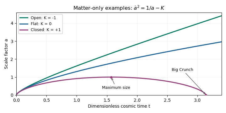
Matter-only scale-factor evolution: closed recollapse, flat power-law expansion, and open expansion tending to a constant speed.
Details. 
For the open matter-dominated Friedmann solution, write , so . The present Friedmann equation gives . With and , the expanding equation becomesChoose the hyperbolic substitutionThen and . Their product givesTake the Big Bang to be , , and integrate. The parametric solution isThe parameter is determined explicitly byThus is conformal time multiplied by , with its origin at the Big Bang; it is not equal to unscaled cosmic time. In particular today . Small gives and , hence . Large gives , in agreement with the curvature-dominated universe limit.
A cosmological gauge transformation changes the coordinates used to identify a perturbed spacetime with its homogeneous background. It can produce apparent metric perturbations even in a physically unperturbed FRW metric. For and unchanged time, the inverse differentials are, to first order,Inserting these into the background line element gives the transformed componentsThe spatial components can now depend on position, although no physical density inhomogeneity or spacetime curvature perturbation has been introduced. For a scalar displacement , these are pure coordinate-generated scalar cosmological perturbations: , , and in the transformed coordinates.
The gauge problem is that individual perturbation variables mix this coordinate freedom with physical fluctuations. A nonzero coordinate-dependent field therefore need not represent a physical effect. One must either choose a definite gauge, such as Newtonian gauge in cosmology, or construct invariant combinations, while ensuring that observables do not depend on that choice.
The same invariant interval can be written as . Applying the chain rule to the differentials proves the metric transformation lawFor first-order scalar cosmological perturbations and , compare perturbations at the same background coordinate label. Expanding the Jacobians and the shifted background gives the linear metric gauge-transformation lawFor the background , , the Lie derivative components areHere primes denote conformal time and is the conformal Hubble parameter. These expressions establish all four alternatives, including any chosen pair.
The component is , immediately giving the lapse function perturbation transformation. The component is , giving the shift vector scalar-potential transformation. The trace of the spatial perturbation is , so tracing the spatial Lie derivative gives the transformation of . Its trace-free scalar part is , giving the transformation of . ThusAs usual, identifying scalar potentials from their derivatives uses the standard boundary conditions, or nonzero Fourier modes, to remove homogeneous ambiguities.
At first order, tensor cosmological perturbations are spatial transverse-traceless tensors. The coordinate-generated spatial perturbation consists of a trace term and symmetrized derivatives of the displacement. In Fourier space, the latter terms carry a factor or . The transverse-traceless projector removes these longitudinal terms and the trace, including the derivative of a transverse vector displacement. Therefore the tensor perturbation is gauge invariant at linear order around the homogeneous background. This is a first-order statement, not a claim of automatic invariance at arbitrary perturbative order.
Because density is a scalar field, . Write both sides as background plus perturbation and expand the background time shift:The coordinate shift acting on an already first-order perturbation contributes only at second order. Thus the density perturbation gauge transformation isThe uniform-density curvature perturbation in the paper's sign convention isThe derivative on is essential and is present in the PDF; the TeX transcription drops it. The scalar-curvature combination transforms aswhile the density term changes by . Hence the two time-slicing changes cancel:On a uniform-density slice, and this variable is the signed spatial-curvature perturbation. The construction assumes ; a pure constant-density cosmological constant does not define such a time slicing.
In Newtonian gauge in cosmology, and . The background cosmological perfect-fluid continuity equation gives , so, writing ,Set the cosmological adiabatic sound speed . Then . Differentiate the previous expression and insert the perturbed energy-conservation equation:Consequently the curvature evolution equation in this sign convention isThe last equality defines the total energy-frame velocity by . For adiabatic cosmological perturbations, the non-adiabatic pressure perturbation vanishes. On superhorizon scales, the stated suppression of the velocity divergence makes the remaining gradient term negligible. Thus is conserved to leading order in . The positive sign of the pressure source follows from the paper's definition of and must not be replaced by a formula using the opposite curvature convention.
Superhorizon conservation of uniform-density curvature lets one carry a primordial perturbation from its inflationary generation through otherwise complicated eras and predict the initial conditions for later Cosmic microwave background anisotropy and structure growth. It relies on adiabaticity: an isocurvature perturbation can source curvature evolution, so the same conclusion is not automatic in an arbitrary multifield model.
Consider a species in thermal equilibrium, with energy density and pressure depending on temperature and with vanishing chemical potential, as in the supplied thermodynamic relation. Put . The first law of thermodynamics givesSince ,The differential is therefore exact:After fixing the irrelevant additive entropy zero, the entropy density at zero chemical potential isMore precisely the first law leaves an additive constant in ; extensivity fixes that constant for the usual entropy-density normalization. A nonzero chemical potential would instead require , so the stated formula is not a universal identity for a decoupled massive species with conserved particle number.
For a reversible thermodynamic process that is an adiabatic process in a comoving volume, and the cosmological perfect-fluid continuity equation gives . Differentiating the extensive expression explicitly, or using the exact differential above, givesThis is cosmological entropy conservation for the closed equilibrium gas with no entropy-producing energy injection.
For radiation in cosmology, , so . Comparing and yields the coefficient ratioWhen all relativistic species share the same temperature and count, the familiar normalizations are and . More generally the energy and entropy effective counts can differ; the common here uses the assumptions stated in the question.
Let be the residual gas temperature immediately before decay. This is the that enters the target abundance formula, not the higher reheating temperature after decay. Before the decay, separately conserved relic number and gas entropy give the conserved cosmological relic abundance . The cold nonrelativistic relic has negligible kinetic energy, henceAssume its density dominates over that of the residual gas and that curvature and dark energy are negligible in the Friedmann equation. Using the reduced Planck mass gives . Under the allowed sudden decay of a dominant nonrelativistic relic convention , the temperature immediately before decay isThe coefficient inherits the approximation : the result is a sudden-decay estimate, not an exact age relation for a matter-only universe. If were instead the exact cosmic age in an uninterrupted spatially flat matter era, would replace the numerator by .
The assumptions also require thermal decoupling in cosmology and negligible prior decay so that remains conserved, a fixed relativistic count , and rapid thermalization after the energy release. In the same approximation, the reheating temperature follows from :Its absence of at fixed decay rate makes clear why the two temperatures must be distinguished.
The instantaneous-decay approximation keeps the scale factor and physical volume fixed across the decay. Energy conservation and rapid thermalization giveMeanwhile the abundance relation gives . Dividing yields the entropy-injection factorThere is a numerical error in the printed coefficient: part (c) omits the factor . The denominator supplies that factor, while the radiation energy contributes to the numerator. Thus the consistent coefficient is , rather than . Both cannot follow from the stated part (b) using the same decay-time approximation.
Its increase is especially transparent without dropping the original radiation. Let . At unchanged , , soRelic domination means , so the leading estimate is much larger than one. This is entropy production by decay of a dominant relic.
There is no conflict with part (a). The equilibrium gas before the decay was a separately conserved, reversibly expanding system. During decay it receives energy from the nonthermal relic, and the decay products thermalize irreversibly. Its cosmological perfect-fluid continuity equation now has an energy-injection source, so does not vanish. The assumptions behind cosmological entropy conservation therefore fail during the event. Moreover the zero-chemical-potential equilibrium expression in part (a) cannot be imposed on the decoupled relic as though it were already part of that same equilibrium radiation bath. The Second law of thermodynamics permits, and here requires, the resulting entropy increase.
For either scalar field with mass , the supplied covariant equation in the FLRW metric is the Klein-Gordon equationSince , and , its conformal-time form isThe homogeneous scalar field backgrounds satisfy the same equations without spatial derivatives. After subtracting them, let and . The key derivatives areBecause , the expansion-friction term cancels after this canonical rescaling of a scalar cosmological perturbation. The fluctuation equations areThe quadratic potential has no mixed derivative, and the stipulated neglect of metric perturbations removes gravitational mixing. Thus these two rescaled fluctuations evolve independently in this approximation.
The given symmetric Fourier transform convention sends to , where . Hence the Fourier-mode equations areThey are harmonic-oscillator equations with time-dependent squared frequencies; a negative effective squared frequency for a rescaled field does not itself imply growth of the physical field .
In the constant- de Sitter approximation, with , so . The massive rescaled mode obeysFor a fixed mass in the specified open interval, at sufficiently late superhorizon scales with , the term is negligible compared with the inverse-square term in the limiting equation. Try . The indicial equation is , givingThus both independent branches of the massive de Sitter superhorizon scalar mode are present inThe coefficients are constant in time and fixed by initial conditions. Writing avoids ambiguous fractional powers of the negative number ; a chosen complex phase in the printed notation can be absorbed into the coefficients.
For the specified mass range, . The physical fluctuation is , so its two branches behave as and . Both exponents are strictly positive. Therefore both physical-field branches decay as :The slower branch of itself grows because , but the expanding scale factor more than cancels that growth. A spatially homogeneous background field of this mass satisfies the corresponding equation and also has these decaying powers.
Evaluate the field variance in the zero-occupation Fock vacuum, , with . The canonical commutation relation alone does not specify a quantum state; this vacuum assumption is needed for the requested expression without occupation factors. In the Heisenberg picture, use the position-space mode expansion of a free fieldThis is the position-space form of the shorthand oscillator expansion in the question; equivalently its Fourier operator uses the creation operator with opposite wavevector. The annihilation operators give , while all other vacuum pairings vanish. The mean field fluctuation is zero, so the two-point function is its coincident-point vacuum field variance. Assuming spatial isotropy, angular integration gives the variance per logarithmic wavenumber interval:Here the dimensionless power spectrum is denoted , as in the question, rather than the alternative notation . A coincident vacuum field product needs smearing or ultraviolet regulation: the unregulated full vacuum variance is generally divergent. With a specified finite wavenumber band, the same expression holds with those integration limits. This does not affect the mode-by-mode dimensionless power spectrum.
For the leading nonzero slower branch, put and . Since the physical fluctuation is , its dimensionless power spectrum isFor a -independent coefficient , this is a blue spectral tilt, because in the specified mass range. At fixed it decays as , consistently with the field-amplitude decay found above.
To include the other branch explicitly, the general superhorizon expression isIf , it approaches the displayed target spectrum with . A pure faster classical branch would instead have power proportional to . For a normalized quantum mode, however, the Wronskian normalization requires both independent real solutions; its slower coefficient cannot vanish. Thus the target is the leading superhorizon quantum spectrum, while the faster classical solution remains part of the complete mode analysis.
Articles by others on the same topic
There are currently no matching articles.