Use the extended real numbers . A proper convex function never takes and is finite somewhere. Its effective domain isFor a proper extended-real function, convexity meansThe endpoint cases are identities; taking avoids the ambiguous product . Equivalently, its epigraph is a convex set. In particular, the effective domain is a convex set. Properness is an additional condition: it rules out the identically function and all values, rather than requiring finiteness everywhere.
For , the subdifferential is the set of supporting slopesEach element is a subgradient. Define outside . The defining subgradient inequality must hold globally, not merely in a neighborhood of . For a differentiable finite convex function, .
Write for the infimal convolution. It is proper by the permitted hypothesis. If and are finite, choose within of their respective infima. For , put and . Convexity of and givesLet . If either endpoint value is infinite, the desired inequality is automatic. Thus the infimal convolution is convex, without assuming the infimum is attained.
For its convex conjugate, replace a negative infimum by a supremum and then change variables :The two suprema separate because and are independent. Properness of and makes each supremum strictly greater than , so this separation remains valid when one or both are . Therefore . This is the conjugate of an infimal convolution. The bounded-domain assumption is unnecessary for these two calculations; the assumed properness and lower semicontinuity of will be used when applying subgradient inversion under convex conjugacy.
Use the conventionThis proximal map is also the resolvent of a monotone operator . A proper lower semicontinuous convex function has an affine minorant, so the quadratic term makes this minimization coercive and strongly convex. A unique minimizer exists for every . Its subgradient optimality condition isThe Moreau–Yosida regularisation is . The conjugate of an infimal convolution and the quadratic conjugate giveThe factor here is essential. Apply subgradient inversion under convex conjugacy, followed by the subdifferential sum rule with the everywhere differentiable quadratic:The last equivalence is precisely the unique proximal minimization condition. ThusThis proves both existence and uniqueness of the subgradient, rather than only identifying a possible element. The finite convex function is therefore differentiable, with , the gradient of a Moreau envelope.
For completeness, monotonicity of applied to the two proximal conditions givesHence is firmly nonexpansive. Expanding the same inequality shows that is firmly nonexpansive too. In particular, is -Lipschitz continuous. None of this requires a bounded effective domain; the result applies to the next example as well.
For the Euclidean norm, rotational symmetry and minimizing the radial objective give the radial soft thresholding formulaIndeed, if , an optimal is a nonnegative scalar multiple of ; minimizing over gives . The gradient of a Moreau envelope is consequentlyAt this is , and the two expressions agree when . The Moreau envelope of the Euclidean norm itself isThus a quadratic core replaces the nondifferentiable tip while the outer gradient remains the normalized radial direction. The Euclidean norm has an unbounded effective domain, unlike the earlier bounded-domain hypothesis; the preceding argument explicitly shows that this restriction is unnecessary here.
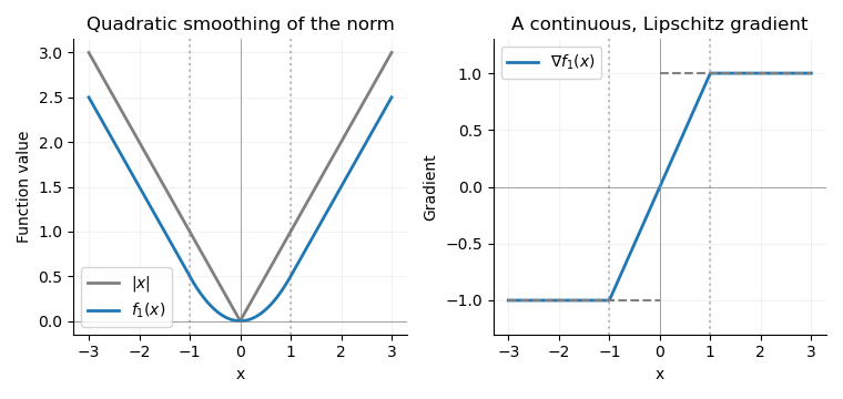
The absolute value and its Moreau envelope with tau equal to one, together with the continuous clipped gradient replacing the jump at the origin
. Details. 
For convex optimization, this Moreau–Yosida regularisation permits gradient descent and other methods for functions with a Lipschitz gradient, using a gradient Lipschitz constant . It approximates the norm uniformly: . Smaller improves approximation but makes the permitted gradient steps smaller. Minimizing alone preserves the minimizers and minimum value of ; replacing one term in a larger objective can shift the minimizer, so the smoothing parameter controls that approximation error.
For , an averaged operator has the formfor some nonexpansive mapping , meaning for all . The word averaging refers to a convex combination with the identity. It does not mean averaging function values over a neighborhood.
An equivalent and useful averaged-operator inequality isTo see it, put and and expandUse and . Conversely, substituting into the same expansion proves its nonexpansiveness from the displayed inequality. The strict range matters for convergence of unrelaxed iterations: a general nonexpansive mapping such as can have nonconvergent alternating iterates.
A firmly nonexpansive mapping satisfiesWriting and , this is equivalent toIt is also equivalent to , so is a nonexpansive mapping. Consequently firm nonexpansiveness is exactly -averagedness. A proximal map of a proper lower semicontinuous convex function is a basic example. A -averaged operator is also -averaged for every , by combining its nonexpansive part with the identity; the equivalence with firm nonexpansiveness specifically uses the parameter .
The Browder convergence theorem for averaged operators states: if is an averaged operator and its fixed-point set is nonempty, then for every starting point, converges in norm to a fixed point of . The theorem assumes a fixed point exists; averaging by itself does not create one.
The finite-dimensional mechanism is worth making explicit. For any fixed point , the averaged-operator inequality givesThis is Fejér monotonicity with respect to the fixed-point set. It makes the sequence bounded and, by summation, makes finite. Hence its residual tends to zero. Choose a convergent subsequence ; continuity of the nonexpansive mapping implies . Apply Fejér monotonicity with . The nonincreasing distances have a subsequence tending to zero, so the whole sequence converges to . This last compactness step uses finite dimension; a corresponding general Hilbert space statement usually gives weak convergence.
Here -smooth means that is differentiable on the entire Euclidean space and has an -Lipschitz gradient, with . Together with convexity, this implies -cocoercivity:First, integration of the Lipschitz gradient along a line segment proves the descent lemma:Indeed, subtract the linear term and integrate for ; its absolute value is at most .
Fix and define . This is a convex function, has the same Lipschitz gradient constant, and , so is a global minimizer. Put . The descent lemma at with givesThereforeInterchange and add the inequalities. The function values cancel, leaving the asserted cocoercivity. This is a proof of the Baillon–Haddad theorem without assuming a second derivative. Convexity is essential: has a -Lipschitz gradient but its gradient is not cocoercive.
Assume , as is necessary for convergence to a minimizer. The printed hypotheses alone omit this condition: in scalar is convex with an -Lipschitz gradient for any prescribed , but has no minimizer, and the update sends to .
Under existence, define the full update . The proximal -step is uniquely defined by strong convexity of its quadratic term and satisfiesThe partial subdifferential in this equation belongs to the scalar function ; differentiating a subdifferential itself would not define the printed proximal minimization.
We prove directly that the alternating proximal-gradient operator is averaged. For two inputs and , setThe input difference is , the output difference is , and the difference of the two update residuals is . Exact expansion givesThe first inequality uses cocoercivity at the mixed points . Therefore is -averaged for the requested . In particular, the endpoint is covered: is firmly nonexpansive, not merely nonexpansive.
A fixed point has and , so the two optimality equations give and . Conversely, at a minimizer both gradients vanish and neither step moves. By convexity,The assumed existence of a minimizer supplies a fixed point. The Browder convergence theorem for averaged operators now givesNo uniqueness of the minimizer is needed. The same estimate even proves averagedness for in this smooth setting, but the requested interval already suffices. The existence condition and the use of the gradient at are both essential to the proof as presented.
Set . Completing the square in the -minimization givesThus, with , the steps in terms of the proximal map of areThe factor comes from the squared residual without a prefactor. The proximal map can equivalently be denoted . Since is a finite convex function, it is continuous, and the quadratic makes the proximal minimizer unique.
A general convex may be nondifferentiable, so this last example need not satisfy the full -smooth hypothesis of the preceding part. The formulas nevertheless remain well-defined: only the derivative is used explicitly. If has an -Lipschitz gradient, one may take in the smooth proof, where is the operator norm.
There is also a useful nonsmooth extension. Put , whose Lipschitz gradient constant is . For two updates, retain the mixed-point differences above, let , and let be the difference of the two selected subgradients of at . The input difference is and the output difference is . Monotonicity of gives . The same norm expansion now yieldsFor , discard the nonpositive term and use . The result is the firmly nonexpansive mapping inequality for the full residual . Fixed points satisfy and , exactly the subgradient optimality condition for the convex objective. Thus the stated algorithm also converges for nonsmooth under this sufficient step bound, provided a minimizer exists; this extension uses monotonicity, not an unavailable gradient of .
Let be a set-valued mapping and let . The Aubin property at means there are neighborhoods of , of , and a finite constant such thatHere is the closed unit ball. Equivalently, every solution near can be matched to a solution within . The localization is on the left-hand side: the matching point need not be in . The property is also called the Lipschitz-like property.
For sensitivity analysis, let represent data or perturbations and the set of feasible or optimal solutions. The Aubin property bounds how far a nearby solution can move when the data change. Taking , also guarantees a nearby solution for each sufficiently small perturbation . It is a stability estimate for a relation, and by itself does not imply uniqueness or differentiability. For a single-valued solution map, it reduces to local Lipschitz continuity.
Work in finite-dimensional Euclidean spaces. Suppose the graph of a set-valued mapping,is locally closed at . Local closedness means that its intersection with some neighborhood of this point is closed relative to that neighborhood. This assumption is part of the criterion.
For a set and , define the Fréchet normal cone byAt an isolated point the condition is vacuous, so all vectors are regular normals. The limiting normal cone consists of limits of these regular normals at nearby points:It can be nonconvex. The Mordukhovich coderivative isThe minus sign in the output-dual component is part of the definition. For a single-valued continuously differentiable mapping , the graph normal is , giving . Thus the coderivative extends a transpose derivative, rather than the ordinary forward derivative.
The exact Mordukhovich criterion isThis is equivalent to excluding a nonzero horizontal limiting graph normal . One must use the limiting normal cone; simply checking regular normals at the reference point can miss normals inherited from neighboring graph pieces.
For sensitivity analysis, apply this test to a solution map or use coderivative and normal cone calculus to express its graph normals through optimality constraints. Triviality of this kernel then proves Lipschitz-like stability without solving the perturbed problem explicitly. Under these same finite-dimensional, locally closed assumptions, the exact Lipschitz modulus is the outer normThe zero-kernel condition is the qualitative criterion; the modulus quantifies the sensitivity bound. For the next problem an explicit local formula is simpler than evaluating these graph normals.
Write the objective as with . Each hinge loss is finite and convex, so the subdifferential sum rule applies without a qualification gap. Its subdifferential isThis formula also covers , if such a sample is allowed, because the loss is then constant. For a convex function, zero in the subdifferential is necessary and sufficient for global optimality. Thus is optimal exactly when there are weights such thatEquivalently, using and ,The notation denotes the segment between and , also when . This avoids reversing interval endpoints for negative-class samples.
Because , the objective is strongly convex, and makes it coercive. It is continuous, so a minimizer exists and is unique for every finite data vector . The weights at exact margins need not be unique even though is. These are the hinge-loss optimality weights for the one-dimensional support vector machine.
Yes: the solution map is locally affine, hence has the Aubin property. Keep the regularization parameter fixed and define the active hinge setSince none of the margins vanishes, the optimality condition at the reference data has no fractional weights:For nearby , define the candidateEach map is continuous and is nonzero at . Because there are finitely many samples, all their signs remain unchanged on a common neighborhood of . Therefore the same set is active at for every . The hinge-loss optimality weights are still on and off , and the defining equation for proves the subgradient optimality condition. Strong convexity makes this candidate the unique global minimizer. Consequently the solution map of a parametric optimization problem satisfiesThis argument establishes stability of the active pattern without presupposing continuity of the unknown optimizer; continuity is used only for an explicit candidate and then optimality is checked.
For , the Cauchy-Schwarz inequality givesThis is the Aubin property with . In fact this constant is the exact local Lipschitz continuity modulus of the affine branch, since its derivative isThe active-set dependence of this derivative is the active-set sensitivity of hinge-loss minimization. At a vanishing margin the affine-branch argument no longer applies, although failure of this particular argument does not by itself prove failure of the Aubin property.

For two scalar samples with alpha equal to one and data (s,1), the optimal coefficient follows two locally affine branches separated by a branch pinned to an exact hinge margin
. Details. 
For the illustration, take , , and with . The hinge-loss optimality weights giveOn the middle branch the first margin is exactly zero, so that branch lies outside the strict-margin hypothesis. The example makes clear why the local affine conclusion is tied to that hypothesis, and also shows that a zero margin need not destroy local Lipschitz stability.
Articles by others on the same topic
There are currently no matching articles.