Let be the rate-of-strain tensor and the Newtonian fluid stress tensor. The viscous dissipation is . The Minimum-dissipation theorem for Stokes flow compares the Stokes flow with every sufficiently regular incompressible flow in the same domain having the same prescribed boundary velocity, with no body force or with a conservative body force absorbed into the fluid pressure. A trial field need not satisfy the Stokes flow equations. Write it as , with and on the boundary. Integration by parts, the symmetry of the Newtonian fluid stress tensor, and giveConsequently the Stokes flow minimizes dissipation:Equality requires a rigid body motion of , which the prescribed boundary eliminates. Extending the flow inside the inserted particle as its rigid body velocity produces an admissible comparison field with zero internal rate-of-strain tensor; hence the extra dissipation due to a rigid inclusion is nonnegative.
Here and below on points into the particle, so the traction represents force exerted by the particle on the fluid. Apply the Lorentz reciprocal theorem for Stokes flow in the fluid region to and the restriction of . The equal outer boundary velocities yieldThe boundary-work formula for viscous dissipation therefore gives . The last integral is zero: is symmetric and divergence-free throughout the particle's original volume, so its total force and torque there vanish, and on is a rigid body velocity. This also allows the sign of this zero-work term to be reversed, giving exactly
With the particle's centre as origin, define , and the particle stresslet tensor . Contracting the linear background velocity with the traction givesThe background rate-of-strain tensor is symmetric and trace-free; the trace of this unprojected particle stresslet tensor does not affect the contraction.
For the straight-rod resistance in a linear flow, write , , , and , . The slender-body force density becomes . The integrals of and are and , respectively, soFor a force-free, torque-free rod, and the perpendicular component of is . Axial spin is not determined by this leading, zero-thickness slender-body theory; it has no effect on . Put . The vector identity givesThe force-free straight-rod orientation equation combines the background rotation with the part of strain that turns the rod; removing preserves its unit length. A rigid body cannot undergo the axial extension or compression imposed by , so opposite axial forces resist that deformation. No leading slender-body force density is needed when , even though the rod may rotate. Its particle stresslet tensor and viscous dissipation are
In the simple shear flow, , and . Thus the rod excess dissipation in shear isThe maxima at correspond to strongest axial extension and compression. The zeros at correspond to zero axial strain: a rod aligned with the velocity or its gradient needs no leading force at that instant. For , with the continuous branch and . Reversing the shear flow reverses the traversal. Substitution givesThe tails make the total finite; the instantaneous zero at lies between two maxima.
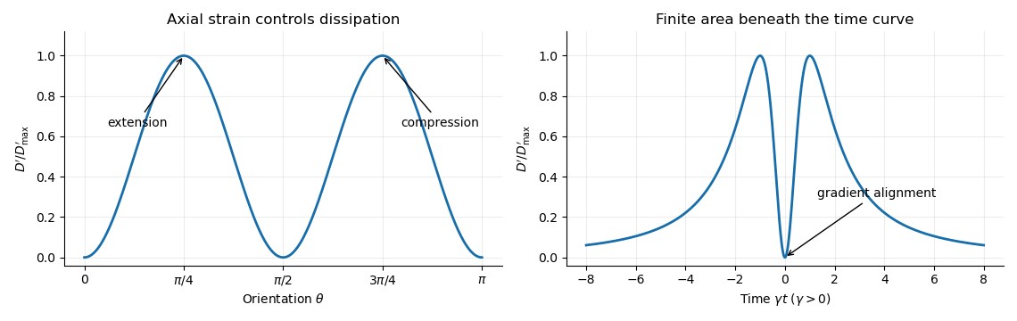

For a dilute rod suspension, the added bulk stress is the number density times the orientation average of the particle stresslet tensor. In this ideal infinitely slender, non-interacting model, rods approach alignment with the shear flow and their excess viscous dissipation decays. A real finite-aspect-ratio rod continues to tumble; rotational diffusion and interactions also maintain a spread of orientations. One therefore expects increased effective viscosity, with alignment offering a mechanism for reduced excess viscosity at strong shear flow. This is a qualitative expectation, not a claim that a finite rod suspension has zero steady excess stress.
In the surfactant transport with exchange relaxation, is the material derivative following an interfacial material element. The term accounts for dilution by tangential stretching, while accounts for changing area through normal motion and curvature. The surface diffusion term redistributes surfactant down concentration gradients. The exchange term relaxes its concentration towards , through adsorption or desorption from a surrounding reservoir, on time scale .
In the bubble frame the spherical interface is stationary and impermeable. A steady material derivative is . For a linear response in the rising speed this and are second order, whereas stretching of is first order. ThusRotational symmetry, linear response to , and zero normal velocity allow only , where is the surface tangent projector. This is the dipolar, axisymmetric sector; axisymmetry alone, without the linear-response assumption, would allow other angular dependence.
On a sphere and . Applying the surface tangent projector to the derivative gives the sphere surface derivative identitiesFor example, taking a second surface divergence of the first identity yields the third. Equivalently, the components of are degree-one spherical harmonics. Hence a dipolar surfactant distribution solves the linear equation:The required smallness condition is . Surface diffusion or exchange must smooth the concentration faster than it is redistributed by the actual interfacial velocity. We require , and ; with neither process there is no such steady linear balance at nonzero . A small capillary number also justifies the spherical approximation.
Take the normal from the inner bubble to the outer liquid, define , and set . The interfacial stress balance with variable surface tension isBecause and , its tangential part becomesThis is a Marangoni stress: surface-tension gradients oppose the clean-bubble circulation.
Use the Unscaled Papkovich–Neuber representation, and . The constant vector potential gives . In the decaying, linear axisymmetric sector, a vector monopole and scalar dipole provide the two constants needed at the sphere; other equivalent potential choices amount to a representation freedom. The PDF potential contains the factor omitted in the TeX aid. With that factor restored, the exterior velocity isAt the interface, no penetration gives , and the tangential velocity gives . Using the traction coefficient printed in equation (3), the tangential stress condition gives . The requested algebraic answers are therefore
There is a factor-of-two error in the PDF traction. Direct differentiation of the preceding velocity with the Newtonian fluid stress tensor givesrather than its printed coefficient . In particular the tangential traction is . Keeping the same definition of , the physically consistent translating surfactant-coated bubble instead has andThe two sets must not be silently conflated. As a useful check, the no-slip limit has the usual total Stokes flow drag with the corrected traction; the printed traction would double it.
Both versions give , , when : the interface is tangentially stress-free and circulates as a clean inviscid bubble. For , , , : the interface is immobile in the bubble frame and behaves as a no-slip sphere. The Marangoni stress remains finite because has a nonzero limit. The concentration smallness condition still has to hold; large is not by itself a complete linearization criterion.
The normal component is balanced by the inner gas pressure and the normal capillary stress , including the variation of , together with the hydrostatic pressure difference responsible for buoyancy. A spatially uniform inner pressure alone cannot balance the dipolar traction. To make the normal stress balance on a translating bubble explicit, let be the outer-minus-inner mass density. After removing the equilibrium Laplace pressure, the corrected outer normal traction has dynamic part . Its degree-one balance isThus, if a terminal speed is desired, , interpolating between the clean-bubble and rigid-sphere speeds. A degree-one shape displacement is merely a translation of the sphere, so the balance determines its rise speed, rather than a dipolar shape distortion.
The hydrostatic approximation gives above the horizontal floor, up to atmospheric pressure. The horizontal Stokes flow equation is , with the no-slip boundary condition at and zero tangential stress on the free surface. Integrating twice gives and the lubrication gravity-current fluxFor the squeegee lubrication model, use vertically, horizontally, and in time. If is the laboratory coordinate in the direction of travel, set , , , and . The blade half-length is . The moving-frame flux is . Conservation of volume gives the dimensionless lubrication equationUsing these scales as representative of the actual flow, lubrication theory requires a small aspect ratio and negligible inertia relative to vertical viscous resistance:The second is the Reynolds number based on , multiplied by . Surface tension is neglected as assumed. Large piles, rounded gaps, and narrow end regions need their own local slope and inertia checks if these representative scales cease to describe them.
For an infinite blade, the steady moving-frame flux is constant and its upstream value is . The infinite-blade gravity pile therefore satisfies , or . Integrating givesAn additive constant in simply shifts . The head at the blade, and hence , must supply the pressure difference that makes the flux beneath the blade equal to the incoming flux. For the deep part has , followed by a smooth transition to with exponentially small, proportional to . Thus is an approximate nose coordinate, not a sharp front of the exact solution.
Near the rounded edge the parabolic lubrication gap is . In the blade frame the floor moves at and the blade is stationary. The Couette-Poiseuille flow in a thin gap has flux . Let be positive leakage towards the rear, and let . The narrow-gap integrals areIntegrating the pressure gradient gives , so the squeegee gap leakage flux isThe first term is the floor-driven contribution. For the steady infinite blade, , so . The hydrostatic pressure difference is the height difference at the two sides. A fully developed rear layer of thickness has moving-frame flux ; hence , andThe large head eventually forces all the arriving film beneath an infinite blade. Taking a perfectly closed gap instead would eliminate this steady state.
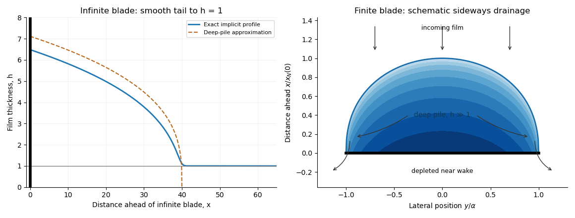
Infinite-blade height profile and schematic finite-blade pile with sideways drainage
. Details. 
For a long finite blade with negligible under-blade flux, fluid accumulates upstream and escapes sideways around the ends. The finite-blade side-drainage pile has in a broad upstream region, while its near wake is strongly depleted; far from the blade the incoming film still has thickness one. The schematic in the preceding figure shows the pile, incoming flow, and escape around the ends.
Away from the nose and end regions, the streamwise flux nearly cancels: . This is the deep part of the infinite-blade gravity pile, so is the appropriate local profile. The hierarchy makes streamwise variation much faster than lateral variation, while allowing lateral flow to carry away the integrated influx.
Set and . Since and the leading deep-pile profile vanishes at its nose, . Integrating steady conservation in gives : the wall has zero normal flux, whereas the matched incoming film supplies flux per unit blade length. Equivalently one can integrate to an upstream matching plane, where the moving-frame flux is exactly ; this avoids incorrectly assigning zero incoming flux to the approximate zero-height nose. Symmetry gives . ThereforeAt leading order the deep pile ends at , so , giving . Direct integration of the cubic profile yields . ThusIn particular and , confirming the assumed hierarchy. The local nose and tip regions are outside this leading deep-pile approximation.
Apply the squeegee gap leakage flux with at most of order the largest pile height. A sufficient negligible-leakage criterion isThe floor-driven must also be small, as it is in this regime. In scaling form the additional restriction is . The total leakage divided by incoming volume flux has the same scaling; blade length does not introduce an extra factor of .
Write , , and choose the common undisturbed interface pressure . The hydrostatic pressure is in the upper fluid and in the lower fluid. Continuity of hydrostatic pressure across both current interfaces givesThus and . This isostatic depth partition of an interfacial current expresses local vertical buoyancy balance: a displaced column with an imbalance would move vertically until the partition was restored. With the hydrostatic pressure subtracted, the pressure within the current is , whereThe equivalent body force is outward for a profile decreasing with . Its magnitude is ; the derivative without an absolute value is a signed quantity.
For an ambient-controlled interfacial plug current, integrating the body force through depth gives radial force per area . The ambient Stokes flow varies over distance , exerting traction , so . The current's internal shear supports the ambient traction with a velocity difference ; requires . The force per area from its in-plane viscous extension is , negligible against ambient traction when . Together these give the viscosity window for an interfacial plug currentFixed volume gives , and the spreading velocity has the scale . Thus andChoosing so that exactly, the similarity solution has , , and . In radial conservation , substitution gives . Regularity and no source at the centre remove the integration constant. Therefore the radial plug velocity is linear:
For the disc-traction analogy for an interfacial current, subtract the imposed straining flow from the stationary-disc solution. The perturbation has velocity on the disc and zero far-field velocity. Reverse its sign: the resulting Stokes flow is driven by a radially expanding disc with velocity in otherwise quiescent fluid. The background straining flow contributes no radial shear traction on , so the given disc traction changes sign. This step uses Linearity of Stokes flow, Uniqueness of Stokes flow, and the no-slip boundary condition. The thin plug current has the same leading boundary velocity and hence the same ambient resistance. Each face contributes ; both faces must be counted. With , radial force balance isIntegrate with . The interfacial plug-current similarity profile isVolume integration gives . Eliminating gives the full prefactor:The formal edge slope diverges, so a narrow edge region lies outside the thin-current approximation. Its traction and volume contributions are integrable, and this is a leading thin-current solution rather than a uniformly valid edge description.
For a diffusion-controlled solute gravity current, excess solute mass, not enriched-fluid volume, is conserved. At late times the effective mass density excess is proportional to solute concentration, so , and . The same ambient resistance scaling givesThis scaling does not determine a universal numerical prefactor. The mass diffusivity controls the growing depth, while dilution weakens buoyancy; assuming a fixed current volume would incorrectly retain the law. The thin-layer requirement becomes ; when only dissolved solute changes the upper fluid, its viscosity is of order the ambient viscosity, consistent with the plug-current window.
Articles by others on the same topic
There are currently no matching articles.