Past exam of the soft condensed matter course of the University of Cambridge / 2021 / Section B / 6

The Flory–Huggins solution theory treats a polymer solution as an incompressible lattice mixture, with one solvent molecule occupying one site and one chain occupying $N$ connected sites. Thus the supplied $f$ is naturally the mixing free energy per lattice site; if a site has volume $v_0$, the free-energy density is $f/v_0$.

The term $k_{B}T(\varphi /N)\ln \varphi$ is the polymer translational entropy of mixing contribution. There are only $1/N$ as many independently translating chains as monomers, which explains the factor $1/N$. The term $k_{B}T(1-\varphi )\ln (1-\varphi )$ is the solvent entropy of mixing contribution. Both lower the mixing free energy for $0<\varphi <1$.

The term $k_{B}T\chi \varphi (1-\varphi )$ is the mean-field excess interaction contribution from replacing like contacts with polymer–solvent contacts. In the simplest energetic lattice model,where $z$ counts neighboring contacts and the ${ϵ}_{ij}$ are pair contact energies. Positive $\chi$ penalizes unlike contacts and can favor demixing. Because chain connectivity suppresses the polymer's translational mixing entropy, relatively modest unfavorable interactions can cause separation of long chains. More general effective $\chi$ can also include entropic effects.

Local compositional stability requires positive curvature of the mixing free energy. Differentiating twice at fixed temperature, with $\chi$ independent of composition as in the given model, givesThe spinodal occurs where this vanishes:Between the two spinodal compositions at sufficiently large $\chi$, $f^{\prime \prime }<0$ and a homogeneous mixture is unstable to infinitesimal composition fluctuations. The binodal is instead fixed by the common-tangent construction, and encloses a larger coexistence region. Between binodal and spinodal the mixture is locally stable but metastable.

A phase diagram with a conventional upper critical temperature additionally assumes that $\chi$ decreases with $T$, for example $\chi =C/T$ with $C>0$. Then high temperature gives a uniform mixture; cooling produces an asymmetric coexistence dome whose critical composition is on the dilute-polymer side. The spinodal lies inside the binodal dome. An arbitrary $\chi (T)$ need not give this orientation, so the free-energy formula alone does not specify a unique temperature axis.

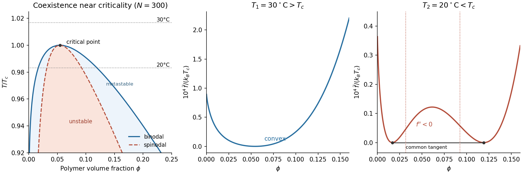
At the thermodynamic critical point, the two spinodal branches merge: $f^{\prime \prime }=0$ and $f^{(3)}=0$. The third derivative isFor $0<\varphi <1$, its zero gives $1-{\varphi }_c=\sqrt{N}{\varphi }_c$. Substitution in the spinodal relation yieldsAn absolute critical temperature requires an interaction–temperature relation. Under the usual energetic approximation $\chi =C/T$, define the theta temperature $\Theta =2C$, at which an infinite chain has $\chi =1/2$. ThenThus $T_c$ tends to a nonzero constant, $T_c\sim N^0$, while $\Theta -T_c\sim N^{-1/2}$. It is the temperature deficit, not $T_c$ itself, that scales as $N^{-1/2}$.

More generally, if a smooth $\chi (T)$ obeys $\chi (\Theta )=1/2$ and ${\chi }^{\prime }(\Theta )\ne 0$, thenThis is the critical point of a Flory–Huggins polymer solution. The same leading chain-length exponent follows for a smooth temperature law, while its coefficient depends on the omitted solvent thermodynamics. The lattice interpretation connects the chain-length dependence of mixing entropy to the theta condition $\chi =1/2$.^[ref].

For $N=300$, the critical polymer volume fraction isIf $v_0$ is the volume assigned to one amino acid in the lattice model, the critical number densities are exactlyThe extra physical approximation needed to use the given radius of gyration is that a chain in a poor solvent is a compact polymer globule. Its size then scales as $R_g\sim b{N}^{1/3}$ with $v_0\sim b^3$, so $N{v}_0\sim R_g^3$. This gives the standard scaling estimatesWith $R_g=3\mathrm{nm}$, numerical substitution givesUsing only the leading large-$N$ value ${\varphi }_c\sim N^{-1/2}$ gives $6.4\times 10^{26}$ and $2.1\times 10^{24}{\mathrm{m}}^{-3}$, respectively. These are scaling estimates, not geometrically exact densities.

For comparison, a specifically uniform spherical compact protein has the radius of gyration of a uniform sphere, $R_g^2=3R^2/5$, so its physical volume is $V_p=(4\pi /3)(5/3{)}^{3/2}{R}_g^3$. Taking $N{v}_0=V_p$ instead gives $n_{m,c}\simeq 6.7\times 10^{25}{\mathrm{m}}^{-3}$ and $n_{p,c}\simeq 2.2\times 10^{23}{\mathrm{m}}^{-3}$. The factor between these conventions is geometric. The PDF does not give a monomer volume, globule density or shape model, and a radius of gyration alone does not determine an exact molecular volume. The model-independent conclusions are the formulas in terms of $v_0$ and the 300:1 ratio of monomer to protein number density.

Interpret the stated transition as an upper critical miscibility temperature: cooling increases the effective $\chi$ through ${\chi }_c$. Above $T_c$, the homogeneous mixing free energy is convex throughout $0<\varphi <1$, with no two-phase common tangent. Below $T_c$, it acquires a region with $f^{\prime \prime }<0$, bordered by the spinodal. A lower straight line touches the curve at two binodal compositions ${\varphi }_{-}$ and ${\varphi }_{+}$; this common-tangent construction gives the equilibrium polymer-poor and polymer-rich phases.

The precise raw curve need not have two equal minima: subtracting an affine function of $\varphi$ changes reference chemical potentials without changing curvature or coexistence compositions. The free-energy panels above subtract the tangent at ${\varphi }_c$ from the upper-temperature curve and the common tangent from the lower-temperature curve. This makes the common tangent and the convex-versus-nonconvex distinction visible.

If the mean initial composition ${\varphi }_0$ lies inside the low-temperature spinodal region, an arbitrarily small separation into equal-volume regions with compositions ${\varphi }_0\pm \delta \varphi$ changes the mean free energy bySmall fluctuations therefore grow spontaneously: this is spinodal decomposition. Interfacial costs limit very short-wavelength fluctuations, and the polymer-poor and polymer-rich domains subsequently coarsen towards their binodal compositions.

If ${\varphi }_0$ lies just outside a spinodal branch but still inside the binodal, then $f^{\prime \prime }({\varphi }_0)>0$. Small fluctuations increase free energy, so the uniform mixture is metastable. Separation requires a sufficiently large nucleus to overcome the interfacial barrier, followed by nucleation and growth. There is no guarantee that this happens rapidly. If the initial composition is outside the binodal as well, it remains a stable uniform phase after cooling.

For a mean composition in the coexistence interval, conservation of polymer fixes the volume fraction $\alpha$ of the rich phase by the lever rule:The temperatures alone do not determine which mechanism occurs without the initial composition. Numerical free-energy curves additionally require $\chi (T)$; the plotted example uses $\chi (T)={\chi }_c{T}_c/T$ with absolute temperatures $T_c=298.15\mathrm{K}$, $T_1=303.15\mathrm{K}$ and $T_2=293.15\mathrm{K}$.