In the weak-field reptation regime of agarose gel electrophoresis, the electrophoretic mobility of a long linear DNA chain scales as , where is its number of base pairs. One way to see the scaling is that the constrained-chain diffusion coefficient scales as , whereas its effective electric charge scales as ; the drift response is proportional to . With the same electric field and running time, the migration distance is therefore . The time cancels from the ratio, givingHere “kbp” means a thousand base pairs, not a rate. The second gel band has traveled farther and corresponds to the shorter chain under this migration model. The inverse-length law applies only over an appropriate migration regime.[ref].
At very low agarose concentration the mesh becomes too open to sieve these chains effectively. In the free-solution limit the chain's electric charge and friction are both approximately proportional to its length, so both chains have nearly the same electrophoretic mobility and their gel bands cease to separate well. At very high agarose concentration the pores become small and transport is strongly hindered; over a fixed experimental time both chains migrate very little, so their absolute spatial separation again becomes small. Increasing gel concentration can improve resolution over an intermediate range, but not indefinitely.
The numerical result is conditional on the inverse-length reptation law. Actual gel electrophoresis size calibration often uses an empirical approximately linear relation between distance and over a specified range. One known band alone cannot fix that relation's slope. The PDF supplies neither gel concentration nor a calibration curve, so is the standard model estimate rather than a uniquely calibrated experimental size.
Choose a coordinate measured from the sphere centre towards increasing distance from the block, so an atom in the sphere is at height . Summing the atom–block potential energy with the sphere's number density givesFor , a uniformly valid Taylor series over the sphere isThe odd moments vanish by reflection symmetry. The sphere volume is , and its second moment isConsequentlyThe first finite-radius correction is therefore . There is no relative correction because the first moment about the centre is zero. The leading term is just the number of sphere atoms times the potential at its centre; the correction increases the attraction because the nearer atoms contribute more strongly than the farther atoms lose.
This is the far-field sphere-plane dispersion energy, with Hamaker constant . It must be distinguished from the near-contact sphere-plane dispersion force, whose small parameter is the surface gap divided by the radius. Here is explicitly the centre-to-plane distance.
Let increase down the pipe, be its radius and the distance from its axis. For steady, fully developed laminar flow of a Newtonian fluid, the axial Navier-Stokes equations reduce toWrite . Integrating twice, regularity at excludes a logarithmic term, and the no-slip boundary condition gives the Hagen-Poiseuille flow profileThe volumetric flow rate follows by integrating over the circular cross-section:For the intended gravity-driven case with no imposed axial pressure gradient, . Substitution givesandThe corresponding mean speed is about and the diameter-based Reynolds number is , consistent with laminar flow. The original PDF does not specify inlet and outlet pressures. If they impose an additional pressure gradient, the general result with above applies; gravity alone does not determine that extra contribution.
Use a rheometer, for example a cone-and-plate rheometer or a parallel-plate rheometer, to impose a small deformation and measure the required torque, or impose a torque and measure the deformation. The apparatus geometry converts these into shear stress and strain. First check that reducing the imposed amplitude does not change the normalized response; this identifies the linear regime and avoids yielding or structural rearrangement.
Three complementary protocols characterize the material's memory. In a stress relaxation experiment impose a small step and hold the deformation fixed. The output is the relaxation modulus , revealing how stored stress decays and whether an elastic plateau remains. In a creep compliance measurement impose a small stress step and record . Removing the load also distinguishes recoverable deformation from permanent flow.
In small-amplitude oscillatory shear, impose sinusoidal strain over a range of frequencies and measure both stress amplitude and phase. With , fitThe outputs are the storage modulus and loss modulus , or equivalently amplitude ratio and loss tangent . These measure elastic storage and dissipative response, respectively. The step experiments give time-domain information and the oscillatory experiment gives the corresponding frequency-domain response. All comparisons must use the same deformation convention and controlled temperature.
The dynamic modulus, or complex viscoelastic modulus, is the ratio of complex stress amplitude to complex strain amplitude in the periodic steady response:This defines the sign convention; for passive response the loss modulus is nonnegative at positive frequency. A Newtonian fluid obeys , while a Hooke's law solid obeys . HenceThe first is purely dissipative and the second purely elastic. Here denotes the scalar deformation used in the problem, with any shear-versus-extension geometric factors already included in its modulus and viscosity.
Parallel elements have the same strain, while their stresses add. The spring supplies and the viscous element supplies , so the Kelvin-Voigt model has constitutive equationFor the oscillatory deformation this givesPhysical stress and strain are the real parts of these expressions. Thus the storage modulus is , independent of frequency, and the loss modulus is . The equation is the quasistatic material law; an inertial equation for an attached mass would require additional mechanical data.
For elements in series the stress is common and the strains add. If and are the Kelvin element and added spring amplitudes, thenThe compliances therefore add, yieldingThis is a standard linear solid model. DefineWriting , its storage modulus and loss modulus areThus increases from the low-frequency plateau to the high-frequency plateau . The loss modulus has low-frequency slope and high-frequency slope on a log-log plot, with maximum at . At that frequency . There need not be a crossing of the two curves for arbitrary spring constants.
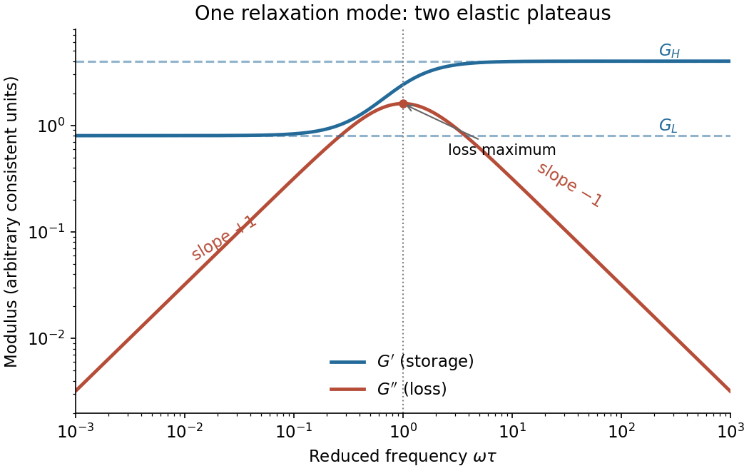

A Kelvin-Voigt model has no finite instantaneous elastic compliance: the viscous element prevents a sudden deformation under a finite stress step. Its creep compliance isConversely an ideal strain step requires an impulsive stress,After the impulse the held-strain response is simply constant. There is no finite stress-decay interval, and the loss modulus grows without bound as . This fails to represent a material with both a finite instantaneous stiffness and delayed stress relaxation.
The added series spring resolves this particular defect. At the instant of loading the Kelvin element cannot move but the added spring can. The standard linear solid model consequently hasandIts instantaneous stiffness is , its long-time stiffness is , and it exhibits genuine stress relaxation as well as delayed creep. The creep retardation time differs from the stress-relaxation time . These properties also follow directly from its constitutive equation,It remains an idealized solid with one relaxation mode: it cannot describe unrestricted long-time viscous flow, nonlinear response, or a broad spectrum of relaxation times.
A hydrophobic surface is poorly wetted by water: on a smooth surface its equilibrium contact angle, measured through the liquid, exceeds . A drop therefore tends to bead up, limiting its contact area. Hydrophobicity does not mean that the surface exerts a mysterious repulsive force on every water molecule.
The waxy coating has a largely nonpolar exterior. Water molecules form favorable hydrogen bonds with one another, whereas a hydrocarbon-rich wax surface offers few suitable hydrogen bond donors or hydrogen bond acceptors. Water–surface adhesion is weak relative to water's cohesion. The drop shape minimizes the combined solid–air, solid–water and water–air interfacial free energies, not merely the liquid's exposed area.
In terms of Young's equation, . A contact angle greater than corresponds to : replacing dry surface by wetted surface has an interfacial cost. The balancing liquid interface then favors a small wetted patch. Microscopic leaf texture can amplify the apparent hydrophobicity, especially when it traps air under the drop as a Cassie–Baxter state; the chemistry of a smooth wax layer alone does not guarantee an extremely large apparent angle.
On Teflon, the water drop has an obtuse contact angle and beads up, whereas the oil drop has an acute contact angle and spreads into a shallower patch. For small drops with negligible Bond number, both can be drawn as spherical caps.
To compare shape at equal volume , let denote the generating sphere radius. The cap height and footprint radius areFor a fixed , these relations give a taller, narrower drop for the larger contact angle. The angles are measured inside the liquid, including the obtuse angle of the water drop.
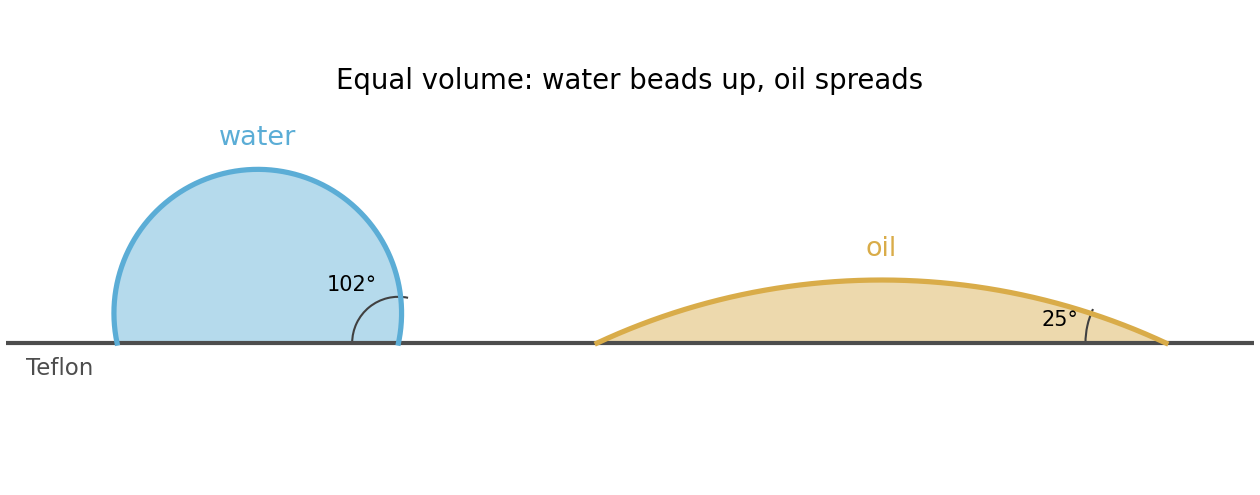

For an ideal smooth homogeneous substrate in thermodynamic equilibrium, Young's equation iswhere denotes air, the solid, and the chosen liquid. It follows either by balancing tangential interfacial forces at the contact line or by varying the wetted area at fixed drop volume.
The dry Teflon–air surface energy is the same in the two measurements, so subtracting the two equations eliminates it:ThereforeThe water–Teflon interface has the higher interfacial free energy per unit area. Neither individual solid–liquid surface energy is determined without the solid–air value; the difference is determined.
Colloidal particles experience attractive Van der Waals forces, arising from correlated molecular charge fluctuations and other dipolar interactions. Integrating many weak molecular attractions over two particles can give a deep near-contact well. For identical spheres of radius and surface gap , a positive Hamaker constant gives approximatelyBrownian motion brings particles into encounters. Without a repulsive barrier, they can reach the attractive primary minimum; if the binding energy is much larger than , thermal motion rarely separates them again. Repeated sticking produces aggregates. This is a kinetic stability statement: thermal agitation causes encounters but does not itself supply a stabilizing interparticle repulsion. The molecular cutoff and hard sphere exclusion prevent the unphysical divergence of the continuum attraction.
One method is to give every particle a sufficiently large surface charge density of the same sign. For example, attach ionizable sulfonate groups covalently to the surface. Dissociation leaves negatively charged surface groups and releases mobile positive counterions into the water. A surfactant with a strongly bound head group can provide another charging route, provided it does not desorb during the experiment.
Each charged particle is surrounded by an electric double layer. As two such particles approach, overlap of these ionic clouds raises the electrostatic and ionic free energy, producing repulsion. In a dilute electrolyte, the range is set by the Debye–Hückel screening length,For identical weakly charged spheres a representative screened Coulomb pair potential isIts sum with the Van der Waals force attraction is the DLVO theory pair potential. Choose the charging level so that the repulsive barrier is many high; particles then rarely reach the primary attractive well during the observation time. This is kinetic stabilization rather than removal of all attraction.
Deionized water is useful because low added ionic strength gives a long-ranged repulsion. It does not mean that the charged dispersion contains no ions: the surface's own counterions are unavoidable and contribute to screening. Surface dissociation, contamination and particle concentration therefore matter even without added salt. An alternative valid route is a dense, firmly attached layer of water-soluble polyethylene glycol, producing steric stabilization without relying on a large electrostatic barrier.
Without stabilization, the potential energy is predominantly attractive outside the molecular core and drops into a deep primary minimum. With the charging treatment, the DLVO theory sum develops a positive barrier between distant particles and that primary minimum. The barrier must be large compared with to inhibit aggregation on the experimental timescale. A shallow secondary minimum can remain at larger separation, depending on parameters.
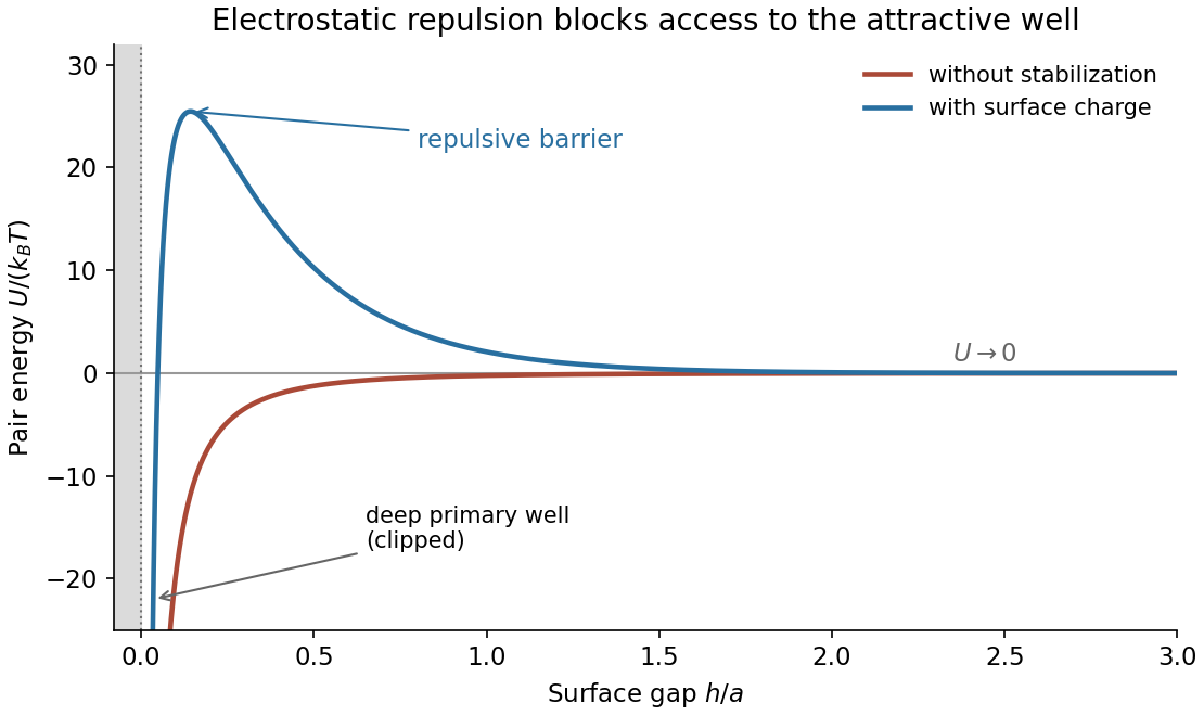
Attractive and electrostatically stabilized colloidal pair potentials
. Original illustrative curves for two equal spheres. The unstabilized curve uses the nonretarded sphere–sphere attraction; the stabilized curve adds screened electrostatic repulsion. The molecular core is excluded and the deep near-contact well is clipped by the plotting range. Potential depths and screening parameters are illustrative, not data supplied by the paper. Details.
The horizontal axis is the surface gap, so the molecular exclusion boundary is at its origin. Both interactions tend to zero at large separation. Raising salt concentration shortens the Debye–Hückel screening length and can reduce the barrier, allowing particles to stick again.
The Flory–Huggins solution theory treats a polymer solution as an incompressible lattice mixture, with one solvent molecule occupying one site and one chain occupying connected sites. Thus the supplied is naturally the mixing free energy per lattice site; if a site has volume , the free-energy density is .
The term is the polymer translational entropy of mixing contribution. There are only as many independently translating chains as monomers, which explains the factor . The term is the solvent entropy of mixing contribution. Both lower the mixing free energy for .
The term is the mean-field excess interaction contribution from replacing like contacts with polymer–solvent contacts. In the simplest energetic lattice model,where counts neighboring contacts and the are pair contact energies. Positive penalizes unlike contacts and can favor demixing. Because chain connectivity suppresses the polymer's translational mixing entropy, relatively modest unfavorable interactions can cause separation of long chains. More general effective can also include entropic effects.
Local compositional stability requires positive curvature of the mixing free energy. Differentiating twice at fixed temperature, with independent of composition as in the given model, givesThe spinodal occurs where this vanishes:Between the two spinodal compositions at sufficiently large , and a homogeneous mixture is unstable to infinitesimal composition fluctuations. The binodal is instead fixed by the common-tangent construction, and encloses a larger coexistence region. Between binodal and spinodal the mixture is locally stable but metastable.
A phase diagram with a conventional upper critical temperature additionally assumes that decreases with , for example with . Then high temperature gives a uniform mixture; cooling produces an asymmetric coexistence dome whose critical composition is on the dilute-polymer side. The spinodal lies inside the binodal dome. An arbitrary need not give this orientation, so the free-energy formula alone does not specify a unique temperature axis.

At the thermodynamic critical point, the two spinodal branches merge: and . The third derivative isFor , its zero gives . Substitution in the spinodal relation yieldsAn absolute critical temperature requires an interaction–temperature relation. Under the usual energetic approximation , define the theta temperature , at which an infinite chain has . ThenThus tends to a nonzero constant, , while . It is the temperature deficit, not itself, that scales as .
More generally, if a smooth obeys and , thenThis is the critical point of a Flory–Huggins polymer solution. The same leading chain-length exponent follows for a smooth temperature law, while its coefficient depends on the omitted solvent thermodynamics. The lattice interpretation connects the chain-length dependence of mixing entropy to the theta condition .[ref].
For , the critical polymer volume fraction isIf is the volume assigned to one amino acid in the lattice model, the critical number densities are exactlyThe extra physical approximation needed to use the given radius of gyration is that a chain in a poor solvent is a compact polymer globule. Its size then scales as with , so . This gives the standard scaling estimatesWith , numerical substitution givesUsing only the leading large- value gives and , respectively. These are scaling estimates, not geometrically exact densities.
For comparison, a specifically uniform spherical compact protein has the radius of gyration of a uniform sphere, , so its physical volume is . Taking instead gives and . The factor between these conventions is geometric. The PDF does not give a monomer volume, globule density or shape model, and a radius of gyration alone does not determine an exact molecular volume. The model-independent conclusions are the formulas in terms of and the 300:1 ratio of monomer to protein number density.
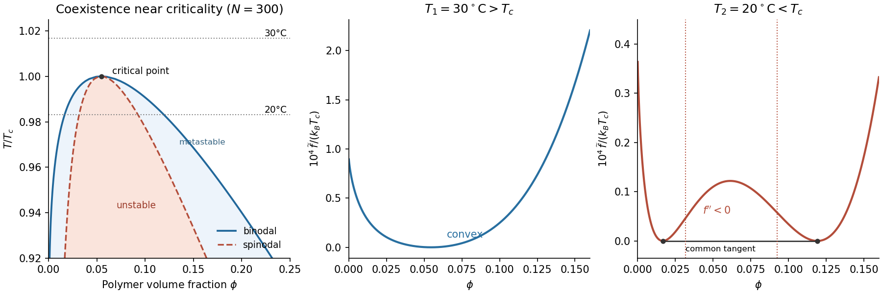
Interpret the stated transition as an upper critical miscibility temperature: cooling increases the effective through . Above , the homogeneous mixing free energy is convex throughout , with no two-phase common tangent. Below , it acquires a region with , bordered by the spinodal. A lower straight line touches the curve at two binodal compositions and ; this common-tangent construction gives the equilibrium polymer-poor and polymer-rich phases.
The precise raw curve need not have two equal minima: subtracting an affine function of changes reference chemical potentials without changing curvature or coexistence compositions. The free-energy panels above subtract the tangent at from the upper-temperature curve and the common tangent from the lower-temperature curve. This makes the common tangent and the convex-versus-nonconvex distinction visible.
If the mean initial composition lies inside the low-temperature spinodal region, an arbitrarily small separation into equal-volume regions with compositions changes the mean free energy bySmall fluctuations therefore grow spontaneously: this is spinodal decomposition. Interfacial costs limit very short-wavelength fluctuations, and the polymer-poor and polymer-rich domains subsequently coarsen towards their binodal compositions.
If lies just outside a spinodal branch but still inside the binodal, then . Small fluctuations increase free energy, so the uniform mixture is metastable. Separation requires a sufficiently large nucleus to overcome the interfacial barrier, followed by nucleation and growth. There is no guarantee that this happens rapidly. If the initial composition is outside the binodal as well, it remains a stable uniform phase after cooling.
For a mean composition in the coexistence interval, conservation of polymer fixes the volume fraction of the rich phase by the lever rule:The temperatures alone do not determine which mechanism occurs without the initial composition. Numerical free-energy curves additionally require ; the plotted example uses with absolute temperatures , and .
Articles by others on the same topic
There are currently no matching articles.