Past exam of the statistics course of the University of Oxford / 2015 / 1

The given probability density function is that of a beta distribution with parameters $r$ and $n-r+1$. We can derive the required moments directly rather than assuming the beta moment formulas. For an integer $j\ge 0$, the Euler beta function givesHere $B(a,b)=(a-1)!(b-1)!/(a+b-1)!$ for positive integers $a,b$; this identity also follows by repeated integration by parts. Taking $j=1,2$ yieldsSubtract the square of the first moment from the second to obtain the variance:These are exact finite-sample identities for each uniform order statistic.

For odd sample size, the sample median is the central order statistic, $M_U=U_{(m+1)}$. Since $n=2m+1$, its index is $r=(n+1)/2$ and $n-r+1=(n+1)/2$. Substitute these into the expectation and variance formulas from part (i):In fact $M_U$ has the symmetric beta distribution $\mathrm{Beta}(m+1,m+1)$, explaining why its expectation is exactly the centre of the interval.

Continuity and strict increase make the quantile function $F^{-1}$ well-defined on $(0,1)$. The endpoints of the uniform distribution occur with probability zero and do not affect the construction. For every real $x$,Thus each $X_i$ has cumulative distribution function $F$. Applying a fixed measurable function separately to independent random variables preserves their independence; explicitly, joint lower-tail probabilities factor asConsequentlyThis is inverse transform sampling. Since $F^{-1}$ preserves order, it also sends the central order statistic to the central order statistic, justifying $M_X=F^{-1}(M_U)$.

First establish the limiting law needed by the delta method. For fixed $t$, put $u_n=1/2+t/\sqrt{n}$ and let $N_n$ count how many of the $U_i$ are at most $u_n$. Then $N_n$ has a binomial distribution with expectation $n/2+t\sqrt{n}$ and variance $n/4-t^2$. The event $M_U\le u_n$ is exactly $N_n\ge (n+1)/2$. Its standardized threshold tends to $-2t$, so the central limit theorem for these binomial counts givesHere $\Phi$ is the cumulative distribution function of the standard normal distribution. Equivalently,Use the usual local regularity for the delta method: $f$ is continuous at the population median $\theta$ and $f(\theta )>0$. The inverse function theorem, applied at $F(\theta )=1/2$, givesThereforeThe asymptotic normality gives the requested leading variance approximationHere the variance parameter for the rescaled limiting law is $1/(4f(\theta {)}^2)$, while the source states the corresponding $1/n$ approximation for the unscaled estimator. Strict increase of $F$ alone does not force $f(\theta )>0$; that local condition is needed for this form of the asymptotic distribution of a sample median.

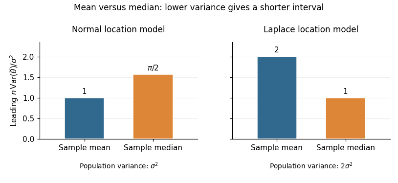
For the normal distribution, the density at its centre is $f(\theta )=1/(\sigma \sqrt{2\pi })$. The sample mean has exact variance ${\sigma }^2/n$, whereas part (b) gives the sample median the leading variance $\pi {\sigma }^2/(2n)$. Thus the requested asymptotic relative efficiency isAt a fixed confidence level, a confidence interval based on the sample mean has a leading half-width smaller by the factor $\sqrt{2/\pi }$. With known $\sigma$, $\overline{X}\pm z_{1-\alpha /2}\sigma /\sqrt{n}$ also has exact normal coverage. Prefer the sample mean under the normal model.

For the Laplace distribution, symmetry puts both the mean and median at $\theta$. Its density there is $1/(2\sigma )$, andConsequently the sample mean has variance $2{\sigma }^2/n$, while the sample median has leading variance ${\sigma }^2/n$. HenceA large-sample confidence interval based on the sample median has leading half-width smaller by $1/\sqrt{2}$; with known scale it is $M_X\pm z_{1-\alpha /2}\sigma /\sqrt{n}$. Prefer the sample median under the Laplace model. Consistent estimation of an unknown scale preserves these leading comparisons. The reason for the reversal is quantitative: the median's precision depends on the central density $f(\theta )$, while the sample mean's precision depends on the whole population variance.