Past exam of the statistics course of the University of Oxford / 2015 (A9, A13765W1)

Source: Mathematics Part A release, member FOI-20210708-1 - Data/a13765w1 (4).pdf. The complete three-page paper is dated 24 June 2015. All thirteen source leaf parts are answered below; the examination statements remain in the private archive.

The department's solution-release policy does not advertise ordinary odd-year solutions. Bounded exact-paper checks on the mathematics and statistics department sites found no matching advertisement of full or selected worked answers, so no source parts are skipped.

The given probability density function is that of a beta distribution with parameters $r$ and $n-r+1$. We can derive the required moments directly rather than assuming the beta moment formulas. For an integer $j\ge 0$, the Euler beta function givesHere $B(a,b)=(a-1)!(b-1)!/(a+b-1)!$ for positive integers $a,b$; this identity also follows by repeated integration by parts. Taking $j=1,2$ yieldsSubtract the square of the first moment from the second to obtain the variance:These are exact finite-sample identities for each uniform order statistic.

For odd sample size, the sample median is the central order statistic, $M_U=U_{(m+1)}$. Since $n=2m+1$, its index is $r=(n+1)/2$ and $n-r+1=(n+1)/2$. Substitute these into the expectation and variance formulas from part (i):In fact $M_U$ has the symmetric beta distribution $\mathrm{Beta}(m+1,m+1)$, explaining why its expectation is exactly the centre of the interval.

Continuity and strict increase make the quantile function $F^{-1}$ well-defined on $(0,1)$. The endpoints of the uniform distribution occur with probability zero and do not affect the construction. For every real $x$,Thus each $X_i$ has cumulative distribution function $F$. Applying a fixed measurable function separately to independent random variables preserves their independence; explicitly, joint lower-tail probabilities factor asConsequentlyThis is inverse transform sampling. Since $F^{-1}$ preserves order, it also sends the central order statistic to the central order statistic, justifying $M_X=F^{-1}(M_U)$.

First establish the limiting law needed by the delta method. For fixed $t$, put $u_n=1/2+t/\sqrt{n}$ and let $N_n$ count how many of the $U_i$ are at most $u_n$. Then $N_n$ has a binomial distribution with expectation $n/2+t\sqrt{n}$ and variance $n/4-t^2$. The event $M_U\le u_n$ is exactly $N_n\ge (n+1)/2$. Its standardized threshold tends to $-2t$, so the central limit theorem for these binomial counts givesHere $\Phi$ is the cumulative distribution function of the standard normal distribution. Equivalently,Use the usual local regularity for the delta method: $f$ is continuous at the population median $\theta$ and $f(\theta )>0$. The inverse function theorem, applied at $F(\theta )=1/2$, givesThereforeThe asymptotic normality gives the requested leading variance approximationHere the variance parameter for the rescaled limiting law is $1/(4f(\theta {)}^2)$, while the source states the corresponding $1/n$ approximation for the unscaled estimator. Strict increase of $F$ alone does not force $f(\theta )>0$; that local condition is needed for this form of the asymptotic distribution of a sample median.

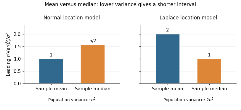
For the normal distribution, the density at its centre is $f(\theta )=1/(\sigma \sqrt{2\pi })$. The sample mean has exact variance ${\sigma }^2/n$, whereas part (b) gives the sample median the leading variance $\pi {\sigma }^2/(2n)$. Thus the requested asymptotic relative efficiency isAt a fixed confidence level, a confidence interval based on the sample mean has a leading half-width smaller by the factor $\sqrt{2/\pi }$. With known $\sigma$, $\overline{X}\pm z_{1-\alpha /2}\sigma /\sqrt{n}$ also has exact normal coverage. Prefer the sample mean under the normal model.

For the Laplace distribution, symmetry puts both the mean and median at $\theta$. Its density there is $1/(2\sigma )$, andConsequently the sample mean has variance $2{\sigma }^2/n$, while the sample median has leading variance ${\sigma }^2/n$. HenceA large-sample confidence interval based on the sample median has leading half-width smaller by $1/\sqrt{2}$; with known scale it is $M_X\pm z_{1-\alpha /2}\sigma /\sqrt{n}$. Prefer the sample median under the Laplace model. Consistent estimation of an unknown scale preserves these leading comparisons. The reason for the reversal is quantitative: the median's precision depends on the central density $f(\theta )$, while the sample mean's precision depends on the whole population variance.

Let $L(\vartheta ;x)$ be the likelihood function, with full parameter space $\Theta$ and null hypothesis $\vartheta \in {\Theta }_0\subseteq \Theta$. The generalized likelihood-ratio test compares the best null fit to the best unrestricted fit:The likelihood ratio $R$ lies between zero and one, and small values count against the null hypothesis; equivalently, large values of the likelihood-ratio test statistic $\Lambda$ count against it.

Compute restricted and unrestricted maximum-likelihood estimates, evaluate their log-likelihoods, and form $\Lambda =2(\ell (\hat{\vartheta })-\ell ({\hat{\vartheta }}_0))$. Under the regular conditions of Wilks theorem, the null limit isThese statistical degrees of freedom count independent parameter restrictions. The regularity includes a locally identifiable smooth model, nonsingular Fisher information, and an interior null value; parameter-dependent support can invalidate the result.

For a chosen significance level $\alpha$, obtain the $(1-\alpha )$ quantile $q_{d,1-\alpha }$ of the chi-squared distribution and useEquivalently, compare the asymptotic p-value $\mathrm{Pr}({\chi }_d^2\ge {\Lambda }_{\mathrm{obs}})$ to $\alpha$. This is a large-sample calibration; part (c) requires direct treatment because its support depends on a parameter.

The count vector has a multinomial distribution, with likelihood functionMaximize its log-likelihood using a Lagrange multiplier for the sum constraint. The equations $n_i/{\pi }_i=\lambda$ and ${\sum }_i{\pi }_i=1$ give $\lambda =n$ and ${\hat{\pi }}_i=n_i/n$. Since all counts are positive and the log-likelihood is strictly concave on the interior of the probability simplex, this is the global maximum-likelihood estimate.

Under the uniform null hypothesis, each category has expected countThe common multinomial coefficient cancels from the likelihood ratio:Taking minus twice its logarithm gives exactlyThere are $k-1$ free category probabilities, because their sum is one, and the null fixes all of them. Thus its regular asymptotic chi-squared distribution has $k-1$ statistical degrees of freedom.

For four categories the number of statistical degrees of freedom is $4-1=3$. The supplied 5% critical value is therefore $q_3=7.82$, and $7.3<7.82$. HenceThe approximate p-value is $\mathrm{Pr}({\chi }_3^2\ge 7.3)\approx 0.063$. This conclusion assumes the large-sample multinomial approximation is adequate, in particular sufficiently large expected category counts. It means there is insufficient evidence against the uniform null hypothesis, rather than establishing that the probabilities are equal.

Write $a=x_{(1)}={\min }_i{x}_i$, $T={\sum }_i{x}_i$ and $\overline{x}=T/n$. For nondegenerate data from the shifted exponential distribution, the likelihood function isFor fixed feasible $\theta$, differentiating its log-likelihood with respect to $\beta$ givesThe derivative changes from positive to negative there. Substituting gives the profile likelihood $e^{-n}(\overline{x}-\theta {)}^{-n}$, which increases with $\theta$. Therefore the unrestricted maximum-likelihood estimates arewhile under the null hypothesis $\theta =0$ the estimate is $\tilde{\beta }=\overline{x}$. Their likelihood ratio isSince the likelihood-ratio test rejects for small $R$, the requested form is obtained withThe formulas assume $\overline{x}>a$, which holds almost surely for a continuous sample with $n\ge 2$; coincident observations give an unbounded unrestricted likelihood and can be treated by its supremum.

An exact calibration is available and also explains why Wilks theorem should not be applied here. Under the null, the memoryless property makes $A=n{X}_{(1)}$ and $D={\sum }_i(X_i-X_{(1)})$ independent gamma distributions with common scale $\beta$ and shapes $1$ and $n-1$. By beta sampling by gamma ratios,Consequently, for $0\le k\le 1$,This yields an exact test size $\alpha$, independent of the unknown scale. The support endpoint and boundary null make this a likelihood-ratio test for an exponential support endpoint, with a different calibration from a regular one-parameter test.

Let $p_0=\mathrm{Pr}(\theta \in {\Theta }_0)$ and $p_1=1-p_0$, assuming both are positive. The prior odds are $\alpha =p_0/p_1$. Given data $x$, the posterior odds areWith conditional joint likelihood $L(\theta ;x)={\prod }_{i}f(x_i\mid \theta )$, define the hypothesis-conditional marginal densitiesThe Bayes factor for $H_0$ relative to $H_1$ is $B=m_0(x)/m_1(x)$. The normalizations $p_0,p_1$ matter: the prior distribution within each hypothesis must have total probability one. Bayes' theorem now givesConverting posterior odds to posterior probability therefore gives

Take $\sigma ,\tau >0$ to be the positive standard deviations. Multiply the normal likelihood function by the normal prior density. Terms independent of $\theta$ can be absorbed into the normalizing constant:The identity ${\sum }_i(x_i-\theta {)}^2={\sum }_i(x_i-\overline{x}{)}^2+n(\theta -\overline{x}{)}^2$ makes the quadratic term explicit. Completing the square giveswhereThus $\theta \mid x\sim N({\mu }_n,v_n)$. This is normal-normal conjugacy: prior and data precisions add, and the posterior mean shrinks the sample mean towards the prior mean zero.

The symmetric continuous prior distribution gives $\mathrm{Pr}(\theta <0)=\mathrm{Pr}(\theta \ge 0)=1/2$, so the prior odds are one. Therefore the Bayes factor equals the posterior odds. Standardizing the normal posterior distribution, putThen $\mathrm{Pr}(H_0\mid x)=\Phi (-z)$ and $\mathrm{Pr}(H_1\mid x)=\Phi (z)$. The endpoint $\theta =0$ has zero posterior probability, so the strict/non-strict split causes no additional term. HenceIn particular, positive values of the sample mean make this Bayes factor smaller, favouring the positive-mean hypothesis.

The denominator $\Phi (z)$ is positive, soStrict increase of the standard normal distribution function turns this into $z>{\Phi }^{-1}(10/11)$. Since the coefficient multiplying $\overline{x}$ in $z$ is positive, the rejection rule is precisely $\overline{x}>c$, withThe quantile is approximately $1.33518$. Equivalently, the rule requires posterior probability of $H_0$ below $1/11$, because its prior odds are one. The calculation is an instance of the Bayes factor for the sign of a normal mean.