For independent bosonic modes, the canonical commutation relation isFor independent fermionic modes, the canonical anticommutation relations arewhere and . The creation operator is the adjoint of the annihilation operator. In either case the mode's number operator iswith or as appropriate. It measures the mode's occupation number. Its possible eigenvalues areFor fermions, implies , so the number operator is a projection. This expresses the exclusion of double occupation of one fermionic mode. The total particle number is .
Expand the anticommutators using the relations in part (a). The terms with two creation or two annihilation operators vanish, leavingEach Majorana fermion operator is Hermitian and squares to the identity. In particular, , so this expression cannot distinguish an empty mode from an occupied one. A single Majorana operator is its own adjoint and does not supply distinct creation and annihilation operators for such an occupation.
An occupation can instead be assigned after pairing Majorana operators into a fermionic mode. For two distinct Majorana operators ,This is a nontrivial projection operator with eigenvalues zero and one. Thus occupation belongs to a chosen pair of Majorana operators, not to an individual Majorana operator.
Use and . Moving operators from different modes past one another introduces a minus sign. Direct expansion givesThus, for real hopping and pairing parameters,At this becomesUse for time to distinguish it from the hopping amplitude . Each unused Majorana operator anticommutes with both factors in , so commuting it through their product gives two minus signs. Hence . The Heisenberg picture equation therefore givesThese are the two uncoupled Majorana zero modes.
For any two distinct normalized Majorana fermion operators , let . ThenandThe same applies to . Both specified pairs have this form. Moreover, the Majorana operators entering are all distinct from those entering , so every cross anticommutator is zero. ThereforeThus are ordinary fermionic annihilation operators, constructed by a different pairing of the four Majorana operators.
The occupation formula from part (b) givesConsequentlyThe independent occupation numbers are each zero or one. The Hamiltonian is independent of , so its four states haveEach energy admits or ; these states differ by occupancy of the zero-energy mode. The ground energy is for either sign of . These degeneracies refer to the full two-mode fermionic Fock space. If one separately restricts to a fixed global fermion parity, only one state at each energy remains in that parity sector.
For a short-range potential, an incident plane wave of unit amplitude and wave vector has the large-distance scattering wavefunctionThe coefficient is the scattering amplitude. For a central potential it depends only on the scattering angle . The incident probability current is , while the scattered radial current is to leading order. Their ratio givesThese are the differential scattering cross-section and total cross section for elastic scattering with the same incident and outgoing wave number.
The expression is asymptotic: it specifies the outgoing wave's leading term, not its finite-distance radial corrections or its form inside the interaction region. In particular, for angle-dependent , the spherical term by itself has an angular-Laplacian contribution of order to the free wave equation, which is cancelled by subleading terms in the exact solution.
In the first Born approximation, with incident and outgoing wave vectors , put . For elastic scattering,Choose the polar axis along . The angular integral isThe radial Dirac delta distribution then givesThus, introducing the dimensionless shell strength ,The forward value is the continuous limit . This is the delta-shell Born amplitude, with its angular dependence expressed through the momentum transfer.
Away from the shell, the reduced radial equation is free. Regularity at the origin and the definition of the S-wave phase shift giveThe reduced radial wave function is continuous at ; otherwise its second derivative would contain a delta derivative not present in the equation. Integrating the equation across the shell gives the jumpDivide by the common shell value and substitute the two free solutions. This yieldsIf the shell value vanishes, use the undivided matching equations or a continuous limit rather than this logarithmic-derivative division. For an explicit phase shift of a delta-shell potential, write and . The cotangent addition formula givesThe phase is defined modulo ; choose its branch continuously as energy or coupling varies. At zero coupling the physical phase shift is zero.
The scattering length is . Since and , the exact phase shift gives, away from the pole,Thus plot against , so that both axes are dimensionless.
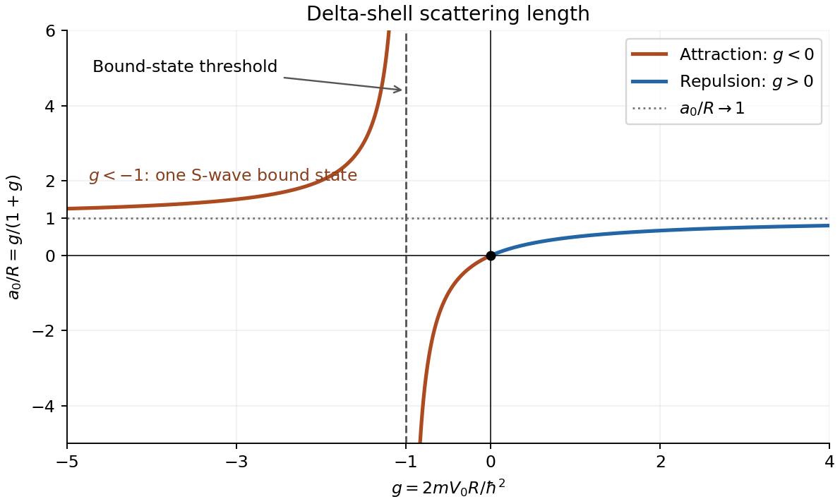
Delta-shell scattering length versus dimensionless coupling, with the bound-state threshold at g = −1
. Details. 
For repulsion, , the curve rises from zero to the horizontal asymptote , staying between zero and one. For weak attraction, , the scattering length is negative and tends to as . For stronger attraction, , it is positive and greater than , tending to as and to as . Its only zero is .
The pole at is the zero-energy threshold of an S-wave bound state. To see this directly, use inside and outside for energy . The same derivative jump givesThis approaches as and admits a positive for . At the threshold the scattering length diverges; this is a zero-energy scattering resonance, not a divergence of the finite-energy cross-section beyond its partial-wave unitarity bound. These are the main features of the scattering length of a delta-shell potential.
The delta-shell Born amplitude is first order in the potential strength:It retains finite-energy angular dependence and includes the leading weak-coupling contributions of all partial waves. By contrast, the supplied is the zero-energy limit of the exact S-wave scattering amplitude. It is isotropic, depends nonlinearly on , and captures the scattering-length pole missed by first-order perturbation theory.
At finite energy the exact S-wave amplitude is insteadwhich is generally complex and obeys elastic unitarity. Its zero-energy limit is for finite scattering length. Thus the two expressions printed in the question represent different approximations; the energy-independent S-wave expression is not the full finite- result of part (c).
Their common regime requires both weak coupling and low energy:Then , soConsequentlyin that joint regime. Low energy alone does not remove the nonperturbative denominator , while weak coupling alone does not remove higher-partial-wave angular dependence.
An ensemble with normalized quantum states and probabilities , , has density matrixEach rank-one projector is Hermitian, so . Taking the trace in any orthonormal basis givesIt is also positive: . Its eigenvalues are therefore nonnegative and sum to one. Hencewith equality exactly when one eigenvalue is one and the others are zero. Thus the purity of a density operator distinguishesEquivalently, a pure state has and rank one. In a -dimensional Hilbert space, purity is at least , attained by the maximally mixed state .
The fixed-particle-number sector is spanned by and . In this basis,The relevant quantum Gibbs state is normalized within this two-dimensional sector, not over all particle numbers. With and , the exponential of a Pauli vector givesThereforeIts eigenstates are , with energies and probabilities . These are nonnegative and sum to one, so the matrix is Hermitian and has trace one. Its purity of a density operator isFor , the zero-temperature limit is the pure ground-state projector,with purity one. As , and , with purity . At every strictly positive finite temperature and finite , both eigenvalues are nonzero, so the state is mixed. If , the two levels are degenerate and the Gibbs state is at all temperatures, including its zero-temperature limit.
Using dimensionless Von Neumann entropy, , givesFor nonzero , as , while as . More precisely, the high-temperature expansion is , and the low-temperature form is . The thermodynamic entropy includes an overall factor .
Fix the mode ordering with the operator before the operator, as in the given state. In the sector with one fermion in each subsystem, use the ordered basisThe state vector is , whose squared norm is one. Thus the global density matrix is the rank-one projectorIt has trace one and satisfies , so the global state is pure.
Take the partial trace over . The conditional vectors in are for and for . Therefore the reduced density matrix isIts determinant is , giving eigenvaluesBoth are positive; in particular, , so the reduced state is mixed despite global purity. The entanglement entropy is obtained by diagonalizing this reduced matrix and evaluatingFor a globally pure bipartite state this equals the entropy of either reduced subsystem. No numerical evaluation is needed.
Using , the Heisenberg picture equations for the quantum harmonic oscillator areSolving these coupled linear equations givesThe oscillator annihilation operator and creation operator areThey obey and . Substitution of the position and momentum solutions, or the corresponding commutators with , yields
Complete the square, keeping the equilibrium displacement signed:Write for position relative to the new minimum. By the sudden approximation, the state immediately after the quantum quench is still the old vacuum. Its initial means areThe old ground state has and . Thus , but the energy measured above the new potential minimum isThe extra term is the excitation energy above the new ground state; the zero-point term remains part of the energy above the potential minimum.
The variables obey the oscillator equations in part (a). Using the above initial means givesThe wavepacket's centre therefore oscillates about the new equilibrium, beginning at the old origin with zero mean momentum.
Define the signed dimensionless displacementThe spatial translation operator is , and the phases of the new energy eigenstates are fixed by . Their expansion coefficients are thereforeSince ,Set and . Their commutator is , which commutes with both operators. Thus the stated special case of the Baker--Campbell--Hausdorff formula is applicable and givesBecause ,Taking the overlaps with therefore provesThis is the coherent state after shifting an oscillator equilibrium. Its normalization follows from .
There is a sign qualification in the printed expansion: agrees with when , equivalently . For a general signed displacement , the odd coefficients have the opposite sign in the specified translated basis. The squared displacement alone fixes the occupation probabilities, not these coherent relative phases. The two-exponential identity also requires the central-commutator condition used above; it is not valid in that simple form for arbitrary operators.
The annihilation operator associated with the new coordinate isAs the initial state is the old vacuum,Equivalently, applying to the number-state expansion in part (c) and shifting its summation index returns times the same state. It is therefore a coherent state of the displaced oscillator.
The new Hamiltonian is . In the Schrödinger picture its evolution givesConsequentlyThe displayed prefactor is only a global phase. Equivalently, in the Heisenberg picture . The mean occupation is constant, and reproduces the energy above the new minimum found in part (b). Its mean position and momentum likewise reproduce that part's oscillating wavepacket centre.
Articles by others on the same topic
There are currently no matching articles.