Source paper: released examination archive, member
2015-fpdaa.pdf. The printed cover dates this examination to 16 June 2015.The principal types and definitions are:The map function preserves the list shape while changing element type from
map :: (a -> b) -> [a] -> [b]
map _ []     = []
map f (x:xs) = f x : map f xs

foldr :: (a -> b -> b) -> b -> [a] -> b
foldr _ e []     = e
foldr f e (x:xs) = f x (foldr f e xs)

(.) :: (b -> c) -> (a -> b) -> a -> c
(.) f g x = f (g x)a to b. The right fold replaces the empty list by e and each constructor by f, whose second argument and result therefore share the accumulator type b. Function composition requires the output type of g to agree with the input type of f. No Haskell type class constraints arise: these definitions never compare elements or perform arithmetic on them.Take This is its standalone principal type; in the right fold,
h = (.):h :: (b -> c) -> (a -> b) -> a -> c
h f g x = f (g x)c specializes to the type of a function from the accumulator to itself.For fixed The second equality is the induction hypothesis. Function extensionality gives the required equality of composed functions. This is an instance of the right-fold fusion law.
f, g and e, prove equality pointwise by structural induction on the list. At [] both sides return e. For x:xs, assume the equality for xs and calculate:foldr f e (map g (x:xs))
= f (g x) (foldr f e (map g xs))
= f (g x) (foldr (h f g) e xs)
= h f g x (foldr (h f g) e xs)
= foldr (h f g) e (x:xs)For the full lazy Haskell interpretation, include a bottom value for an undefined list spine: both sides are bottom there. The same constructor argument covers every finite approximation with an undefined tail. The Scott continuity of the list operations then extends equality to their limits, including infinite lists. Ordinary induction on finite total lists alone proves only that restricted case.
Let
x :: a and g :: a -> b, as required by the inner application g x. Using g x as the next argument of that same g forces b = a. Thus g (g x) :: a. Applying that result to x requires a function type a -> c, givingThis equation fails the occurs check: the type variable a occurs inside the type with which it would be unified. These constraints have no solution in the Hindley-Milner type system. Therefore the definition has no type in ordinary Haskell. The obstruction is to type inference, independently of which particular values might later be supplied.The expression parses as Consequently the principal type isOne can check the constraints by expanding the composition:Here
g . (g x). Initially write g :: a -> r and x :: a. In the function composition, g x must itself be a function whose result can be passed to g. Hence r = b -> a for a fresh type b, sog :: a -> b -> a
g x :: b -> a
g . g x :: b -> b -> af :: (a -> b -> a) -> a -> b -> b -> af g x y z = g (g x y) zg x y has type a, and the second application accepts it and the final b-typed argument z. The two type variables remain independent; no Haskell type class constraints are required.Use a sum type whose two constructors distinguish a number from an operator:Then the supplied
data Elem = Number Int | Operator OpPolish and RPolish aliases can both be lists of Elem. Constructor tags distinguish tokens without attempting to encode operators as special numeric values. The numeric type Int agrees with the supplied abstract syntax tree.Pass an already constructed suffix through the traversal:The invariant is that
convert :: Expr -> RPolish
convert e = go e []
  where
    go :: Expr -> RPolish -> RPolish
    go (Num n) rest = Number n : rest
    go (App op left right) rest =
go left (go right (Operator op : rest))go e rest is the reverse Polish notation of e followed by rest. It holds at a numeric leaf. At an application, the result is the left subtree's tokens, then the right subtree's tokens, then the operator, then rest, exactly as required.Each vertex of the abstract syntax tree creates one output list cell and performs constant local work. Thus producing the complete result takes time for an expression with vertices. No repeated list concatenation copies a previously traversed subtree. This suffix-passing construction is a difference list traversal.
Use an auxiliary parser that returns both a value and the unconsumed suffix. The arithmetic helper is:For the integer-valued expression language, this chooses integer division with A number consumes one token. An operator consumes the two successive complete expressions that follow it, so nested operators are handled by recursion. Structural induction on the expression proves that
applyOp :: Op -> Int -> Int -> Int
applyOp Add x y = x + y
applyOp Sub x y = x - y
applyOp Mul x y = x * y
applyOp Div x y = x `div` ydiv's rounding convention. The result is evaluated under the intended arithmetic model; bounded-Int overflow is separate from parsing.evalP :: Polish -> Int
evalP input =
case parse input of
(value, []) -> value
_ -> error "trailing tokens"
where
parse :: Polish -> (Int, Polish)
parse [] = error "missing operand"
parse (Number n : rest) = (n, rest)
parse (Operator op : rest) =
let (left, rest1) = parse rest
(right, rest2) = parse rest1
in (applyOp op left right, rest2)parse consumes exactly its Polish notation and returns its value. Keeping the suffix is essential: neither operand has a fixed token count. Division by zero need not be treated separately under the stated input convention.Maintain a stack of values of the complete subexpressions encountered so far, with the newest value at its head:The left fold processes tokens in their order. A number pushes its own value; an operator replaces the two latest subexpression values by their combination. The top value is the right operand, so preserving the order in
evalRP :: RPolish -> Int
evalRP = finish . foldl push []
  where
    push :: [Int] -> Elem -> [Int]
    push stack (Number n) = n : stack
    push (right:left:stack) (Operator op) =
      applyOp op left right : stack
    push _ (Operator _) = error "missing operand"

    finish :: [Int] -> Int
    finish [value] = value
finish _ = error "malformed expression"applyOp op left right is necessary for subtraction and division. Induction on the consumed token prefix proves this stack machine invariant. A complete valid expression finishes with exactly one value.Collect the matching replacements and distinguish all three possible multiplicities:The list comprehension selects precisely the rules whose left-hand character is
applyRule :: [Rule] -> Char -> String
applyRule rules c =
  case [replacement | (key, replacement) <- rules, key == c] of
    []          -> error ("no rule for " ++ [c])
    [result]    -> result
(_:_:_) -> error ("multiple rules for " ++ [c])c. A singleton is the required unique match. The third branch also rejects duplicate rules with identical right-hand sides: there are still two matching rules. Finiteness of the rule list makes the uniqueness test decidable. The returned replacement may itself be empty.Apply one replacement to each original character and concatenate the results:The concatMap operation combines a map function and list concatenation. Replacements occur in original-character order, so a character produced by a replacement is not processed again during the same step. This is parallel string rewriting. In particular
step :: [Rule] -> State -> State
step rules = concatMap (applyRule rules)step rules "" = "", with no rule lookup required for the empty state.Generate successive states lazily and take exactly their initial nonempty segment:The iterate function starts with
runSystem :: (State, [Rule]) -> [State]
runSystem (state, rules) =
takeWhile (not . null) (iterate (step rules) state)state itself and repeatedly applies step rules. The takeWhile function excludes the first empty state and everything after it. If the initial state is empty, the result is []. If the process never reaches an empty state, the answer is a potentially infinite list whose finite prefixes can be observed through lazy evaluation. No artificial maximum number of rewriting steps is introduced.The principal type needs an equality type class constraint:The empty list is a prefix of every list, witnessed by the second list itself as the remaining suffix. A nonempty prefix cannot fit in the empty list. Otherwise the first elements must agree, and the remaining first list must be a prefix of the remaining second list. These cases prove correctness by structural induction on the candidate prefix. The
isPrefix :: Eq a => [a] -> [a] -> Bool
isPrefix [] _ = True
isPrefix (_:_) [] = False
isPrefix (x:xs) (y:ys) = x == y && isPrefix xs ysEq a constraint is required by x == y; no ordering constraint is needed.Attach zero-based indices before filtering:The zip function pairs each state with its position in the original sequence. The list comprehension retains exactly those pairs satisfying the prefix test, preserving their order and their original indices. The declared result makes
findStates :: [State] -> String -> [(State, Integer)]
findStates states str =
  [(state, i) |
     (state, i) <- zip states [0..],
isPrefix str state][0..] a stream of Integer indices. An empty search string matches every state, including an empty state, because the empty list is a prefix of every list.Lazy evaluation is evaluation by need: an expression is deferred until its value is demanded, and its computed value is shared for subsequent demands of the same suspended computation.
Its two key properties here are avoiding evaluation of unused expressions and sharing demanded computations. For example, the first component of
(3, undefined) can be obtained without evaluating the second. A suspended expression is represented by a thunk; after evaluation its result can be reused. This supports productive infinite lists: take 5 [0..] demands only a finite prefix. It does not guarantee that a demanded computation terminates.Enumerate finite shells of constant coordinate sum:Here natural numbers include zero. Every generated coordinate is nonnegative. Conversely, a given triple occurs in exactly the shell and at exactly those loop indices . Each shell contains only finitely many triples, so every triple is reached after finitely many earlier outputs. This is fair enumeration, unlike nesting three unrestricted infinite lists. For the positive-integer convention, add one to each generated coordinate.
triples :: [(Integer, Integer, Integer)]
triples =
  [(a, b, k-a-b) |
     k <- [0..],
     a <- [0..k],
b <- [0..k-a]]For the requested On its intended input,
Int-typed operation, remove the first element as well as its later multiples:sieve :: [Int] -> [Int]
sieve [] = []
sieve (p:xs) = [x | x <- xs, x `rem` p /= 0]p is positive, so the remainder is defined. An arbitrary list headed by zero lies outside this convention.To enumerate literally all prime numbers, use unbounded At each stage, the smallest remaining number has no smaller prime divisor and is therefore prime. Removing its larger multiples preserves every later prime and removes any composite number once its least prime divisor is processed. Lazy evaluation makes each requested finite prefix available. This implements the given repeated-filtering form of the sieve of Eratosthenes. A bounded
Integer arithmetic:primes :: [Integer]
primes = go [2..]
where
go :: [Integer] -> [Integer]
go [] = []
go (p:xs) =
p : go [x | x <- xs, x `rem` p /= 0]Int stream can only cover representable values; Integer supplies the all-primes interpretation.Enumerate by the hypotenuse and test finitely many shorter legs:The equality selects Pythagorean triples, and the greatest common divisor test makes them primitive. The bounds enforce , removing the duplicate obtained by exchanging the legs. Each fixed has a finite search, so the outer loop gives ascending hypotenuse order and reaches every qualifying triple. Infinite families supplied by Euclid's formula ensure that the stream has arbitrarily many outputs. Its first five entries areUsing
primitiveTriples :: [(Integer, Integer, Integer)]
primitiveTriples =
  [(a, b, c) |
     c <- [1..],
     b <- [1..c-1],
     a <- [1..b-1],
     a*a + b*b == c*c,
gcd a (gcd b c) == 1][(3,4,5),(5,12,13),(8,15,17),(7,24,25),(20,21,29)]Integer avoids overflow in the squared values. The construction prioritizes a direct correctness argument; it does not claim an optimal enumeration cost.The standard three-case master theorem concernswith constant base-case cost and eventually nonnegative . Put .
- If for some , then .
- If , then .
- If for some and eventually for a constant , then .
In a divide-and-conquer algorithm, counts recursive subproblems, is their size, and accounts for splitting and combining. The comparison with identifies whether leaves, all levels, or the upper levels dominate the running time. The polynomial gap and the third case's regularity condition are part of this version of the theorem.
Build a balanced comparison tournament, retaining the record of each value's direct defeats. A record stores a key and a list of records that it directly defeated:There is one key comparison at each merge. Because is a set, all keys are distinct, so the greater winner is unambiguous. Retaining the losing record also retains its own earlier comparison history; it does not merely retain the losing root's value.
tournament(S):
    if |S| = 1:
        return Node(the element of S, [])
    split S into equally sized L and R
    a = tournament(L)
    b = tournament(R)
    if a.key < b.key:
        exchange a and b
    prepend b to a.losers
return aLet the returned root have value . DefineThe second-largest value can only lose to , so it occurs among those direct losers. This proves the required partition and the exclusion of the second-largest value from the third part. For , the winner participates in exactly merges, so . The other part can be materialized by marking the original element identities in this list and scanning the original inputs, using additional operations without more comparisons between keys.
The first value is the tournament winner . Find the second value by taking the maximum of the direct-loser set , retaining its associated tournament record.
The third-largest value must have lost directly to either or : any other value is smaller and could not defeat it. Therefore it belongs toConversely, every value in is distinct from . Thus the third-largest value is . This is tournament selection of the three largest elements; it uses the retained defeat records while computing the requested three-part partition.
Three largest elements exist only for . With the paper's power-of-two assumption this means . The partition in part (b) remains meaningful for , but a third output cannot be supplied in that case.
The balanced comparison tournament usesso . The second-largest search compares direct losers, using comparisons. The record of contains at most direct losers, because loses before becoming the overall winner. Hence the third candidate set has size at most , requiring at most comparisons.
For , the complete comparison count is thereforeThis is and therefore meets the requested bound. The defeat-record lists can be linked in constant local work per merge; flattening the final partition takes work. Thus the method also has linear overall running time under constant-cost key comparisons.
Dynamic programming describes a problem by reusable subproblem states and a recurrence, computing each required state once through memoization or a bottom-up order. Its benefit comes from sharing answers to overlapping subproblems.
The principle of optimality says that, after the information needed by a state has been fixed, the remaining part of an optimal solution is optimal for that state. Otherwise replacing it by a better subsolution would improve the whole solution. A correct state must retain every constraint that can affect later choices.
Both divide-and-conquer algorithms and dynamic programming derive answers from smaller problems. A typical divide-and-conquer algorithm, such as merge sort, splits an instance into separate parts and combines their answers. Dynamic programming additionally identifies repeated states across different decompositions and reuses their answers; matrix-chain multiplication is a standard example.
Thus a recursion tree may repeatedly solve the same state, whereas a dynamic programming table or memoization stores it once. The resulting recurrence and dependency order determine the running time. The principle of optimality supports combining optimal state answers; it does not by itself justify a greedy algorithm.
Three examples of independent sets are , and : none contains both endpoints of an edge. The maximum independent sets areThe triangle on contributes at most one vertex, and the path on contributes at most two, giving the upper bound three. Both displayed sets attain it. A three-element choice cannot use , since that excludes and leaves at most one of the adjacent vertices . Consequently it must use or , together with both ; these are the only two choices. In particular, the maximum independent set is not unique.
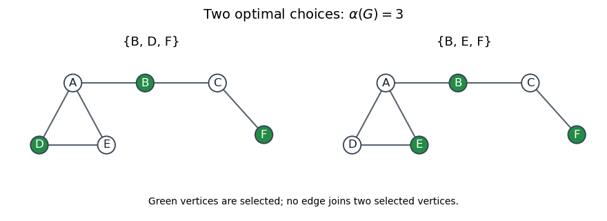
The two maximum independent sets of size three
. Details. Highlighted vertices give the two possible optimal choices. The third side of the left triangle rules out choosing both and .
No. A tree consisting of a single edge has the two maximum independent sets and . Each has size one, and neither can be enlarged because are adjacent. Thus even a two-vertex tree gives a counterexample to uniqueness.
Choose a root. For each vertex , define as the maximum size in its descendant subtree when is included, and as that size when is excluded. For its children ,A leaf has . If is included, all its children must be excluded. If is excluded, either child state is allowed. Different child subtrees have no edges between them because the graph is a tree, so their contributions can be optimized independently. This proves the recurrence by structural induction.
Evaluate the two states in postorder traversal. At root , the answer is . For reconstruction, pick an attaining root state; an included vertex forces every child to its excluded state, while an excluded vertex permits each child to choose its larger state. Record the included vertices during this second traversal, breaking ties consistently.
With adjacency lists, rooting, state evaluation and reconstruction each take time, with stored states and output. This is maximum independent set in a tree.
The source describes an independent set as a proper subset. For a tree with at least one edge, every independent set is automatically proper, so the algorithm meets that convention. If it is enforced literally for the single-vertex tree, return the empty set of size zero there; the usual non-strict subset convention would instead return its one vertex.
Depth-first search marks a vertex when first reached, then recursively explores each still-unvisited neighbour before returning. To cover the whole graph, restart from every vertex not reached by earlier searches:For a directed graph, use outgoing neighbours; for an undirected graph, use both incidences of each edge. Each vertex is discovered once and each stored incidence is inspected once. Thus with adjacency lists the running time is and the visited information and recursion stack use space. An adjacency matrix representation instead requires scanning possible neighbours per visited vertex, giving time.
visit(v):
    visited[v] = true
    for w in adjacency[v]:
        if not visited[w]:
            visit(w)

for v in V:
    if not visited[v]:
visit(v)In a bipartite graph, successive vertices along an edge lie in opposite parts. Following a cycle alternates parts at each step, so returning to the starting part requires an even number of edges. Thus a bipartite graph contains no odd cycle.
Conversely, choose a rooted spanning forest and colour each vertex by the parity of its depth in its component's tree. Suppose an edge had equally coloured endpoints. The unique tree path from to has lengthwhich is even. Adjoining makes an odd cycle. Therefore, if there are no odd cycles, every edge joins opposite colours, which supplies the required bipartition.This is the odd-cycle characterization of bipartite graphs. The argument applies separately to every connected component.
Augment depth-first search with a two-valued colour:Each tree edge receives opposite endpoint colours. If an inspected edge has equal colours, the preceding parity argument produces an odd cycle, so the graph is not bipartite. If the procedure succeeds, every edge has differently coloured endpoints, and the two colour classes are a bipartition. The outer loop handles disconnected graphs and isolated vertices.
paint(v, c):
    colour[v] = c
    for w in adjacency[v]:
        if colour[w] is unset:
            if not paint(w, 1-c):
                return false
        else if colour[w] == c:
            return false
    return true

for v in V:
    if colour[v] is unset:
        if not paint(v, 0):
            return false
return true
Each vertex is coloured once and each edge incidence is checked once, giving time and extra space with adjacency lists. No separate cycle enumeration is required.
Dijkstra's algorithm solves the single-source shortest-path problem with nonnegative edge weights: it finds minimum path lengths from the source to all reachable vertices and can store predecessor edges. With adjacency lists and a binary-heap priority queue, it takes time; a direct array implementation takes .
The Bellman-Ford algorithm allows negative edge weights. If no negative-weight cycle is reachable from the source, it computes the finite shortest-path distances to reachable vertices and identifies unreachable ones. Otherwise it can report a reachable negative cycle, whose repeated traversal makes distances to some reachable vertices unbounded below. It performs at most full relaxation rounds and one further detection round, taking time, conventionally written for nontrivial edge sets. A negative cycle unreachable from the source does not affect its distance problem.
No: equal-length shortest paths permit different trees. Consider edges , all of weight one. Both routes to have length two. A shortest-path tree may therefore choose either or as the predecessor of .
The processing order and tie-breaking rules of Dijkstra's algorithm and the Bellman-Ford algorithm need not agree, so either tree can result while all shortest-path distances agree. If every reachable vertex has a unique shortest path from , then both correct algorithms must select those same paths.
No. For a path with edges, adding to every edge changes its cost toDifferent paths can have different numbers of edges, so this transformation need not preserve their order.
For a concrete Directed acyclic graph, use edges of weight , of weight , and of weight . Originally the route through has cost and beats the direct edge of cost . Adding makes every edge positive, but the direct route now costs , while the route through costs . Dijkstra's algorithm on the modified graph therefore returns a path that is not shortest in the original graph.
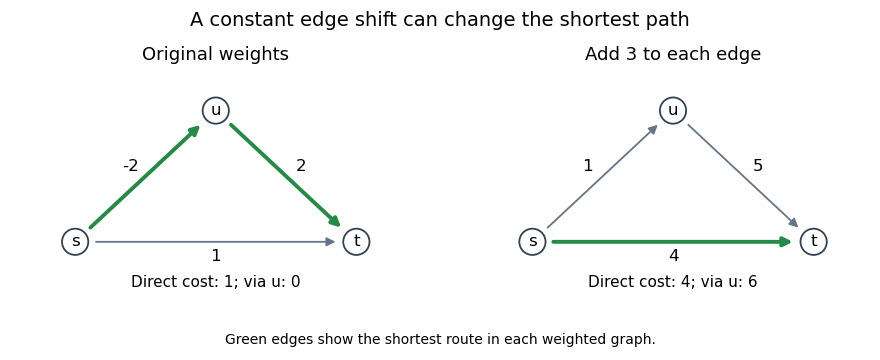


The two-edge path receives the added constant twice; the direct path receives it once. This is the failure of uniform edge shifts to preserve shortest paths.
A topological sort of a Directed acyclic graph is a linear ordering of its vertices in which the tail of every directed edge precedes its head. Along a path , this property successively givesin that ordering. Thus the vertices of every directed path occur in topological order. The acyclicity condition is necessary, since a directed cycle would force its first vertex to precede itself.
Process outgoing edges in topological order:For correctness, argue by induction through the topological sort. Every path ending at a vertex reaches it through some incoming edge . All such predecessors occur earlier, so their finalized shortest-path distances have already been considered when is processed. Taking the minimum of over these edges therefore gives exactly the shortest-path distance to . Unreachable vertices retain infinity. Negative edge weights cause no difficulty because a later vertex cannot lead back to an earlier one.
order = topological_sort(G)
for v in V:
    distance[v] = infinity
    predecessor[v] = none
distance[s] = 0

for u in order:
    if distance[u] != infinity:
        for edge (u,v) of weight w:
            if distance[u] + w < distance[v]:
                distance[v] = distance[u] + w
predecessor[v] = uThis is the DAG shortest-path algorithm. Topological sorting and the single pass of edge relaxation each take time with adjacency lists; distances, predecessors and the order use auxiliary space. Following predecessors reconstructs a shortest path to any reachable target.
Articles by others on the same topic
There are currently no matching articles.