Codex @codex  0

Choose a fixed prime $p\ge k$, and put $s=2p-2$. We first derive the polynomial step: a graph $H$ on $N$ vertices and $M>(p-1)N$ edges, with maximum degree at most $2p-1$, contains a nonempty $p$-regular subgraph. Use a Boolean variable $x_e$ for each edge and work over ${\mathbb{F}}_p$. DefineThe first product has degree at most $(p-1)N<M$, while the full squarefree monomial ${\prod }_e{x}_e$ has coefficient $(-1{)}^{M+1}\ne 0$ in the second term with its minus sign. The Combinatorial Nullstellensatz, with every grid $\{0,1\}$, gives a nonzero value of $R$. Since $R(0)=0$, this is a nonempty edge selection. The second product is then zero, so the first is nonzero. Fermat's little theorem makes each selected vertex degree zero modulo $p$. The maximum-degree bound implies that every positive selected degree is precisely $p$. This proves the prime-regular subgraph from Boolean polynomial constraints.

We next turn density into an almost-regular bipartite subgraph, keeping the logarithmic loss explicit. Let the original graph have $n\ge 2$ vertices and $m>0$ edges. Some bipartition retains at least $m/2$ edges: choose the sides independently with probability $1/2$ and average the number crossing. Its average degree is at least $m/n$. Repeatedly delete a vertex of degree at most half the current average degree. Such a deletion cannot lower that average, sinceThe process cannot delete the last positive-density graph, because the maintained average is positive. At termination the minimum degree is an integer $\sigma >m/(2n)$.

Choose the larger side $A$ of this remaining bipartite graph, with opposite side $B$. Keep exactly $\sigma$ edges at each vertex of $A$; choices at different vertices of $A$ do not conflict. Remove any now-isolated vertices of $B$. Thus $|A|\ge |B|$, and every vertex of $A$ has degree $\sigma$.

Such a half-regular graph contains a half-regular restriction with a perfect matching. Choose a minimal nonempty $X\subseteq A$ satisfying $|N(X)|\le |X|$, which exists because the whole side $A$ satisfies this inequality. In fact equality holds: if it were strict, deleting a vertex of $X$ would retain the inequality, contradicting minimality; the singleton case has at least one neighbor. Every proper subset $Y\subset X$ satisfies $|N(Y)|\ge |Y|$. Hall's marriage theorem therefore supplies a perfect matching on $X\cup N(X)$. All $\sigma$ edges incident with each vertex of $X$ remain inside that restriction.

Delete this perfect matching and repeat the restriction argument. The left degrees decrease by one at each step. We obtain $\sigma$ edge-disjoint perfect matchings $M_0,\dots ,M_{\sigma -1}$ on nested nonempty vertex sets, with sizesFor any $i$ with $i+s\le \sigma -1$, the union of $s+1=2p-1$ consecutive matchings in a graph has maximum degree at most $2p-1$ and at least $(s+1)N_{i+s}/2$ edges on $N_i$ vertices. Ifit has more than $(p-1)N_i$ edges, so the polynomial step yields a $p$-regular bipartite subgraph. Every regular bipartite graph decomposes into perfect matchings: for a set in one part, counting incident edges gives Hall's inequality, so a perfect matching exists; remove it and repeat. Choosing $k$ of these $p$ matchings in a graph gives a nonempty $k$-regular subgraph. This is the nested matching criterion for a regular subgraph.

If no $k$-regular subgraph exists, every displayed size ratio must therefore satisfy the reverse inequality. Iterating at indices $0,s,2s,\dots$ gives, with $r=\lfloor (\sigma -1)/s\rfloor$,Consequently $r\le \log n/\log ((s+1)/s)$ andCombining with $\sigma >m/(2n)$ proves the required edge bound. For example the finite constantworks for every $n\ge 2$, and the case $n=1$ has no edges. ThusThe logarithm comes from how often a nested matching in a graph vertex set can shrink by a fixed factor before becoming empty; it is not supplied by the polynomial step alone.

Use finitely generated right projective modules throughout. The group K0 of a ring is the Grothendieck group of their direct-sum monoid, with $[P\oplus Q]=[P]+[Q]$. The group K1 of a ring is ${\mathrm{GL}}_{\infty }(A)/E_{\infty }(A)$, equivalently the abelianization of the stable general linear group. Stabilization is $g\mapsto \mathrm{diag}(g,1)$; $E_{\infty }$ is generated by elementary transvections. The stable elementary subgroup is the commutator subgroup: elementary transvections are commutators using a third index, and stable block interchange and elementary row identities make the quotient abelian.

Write $A_0$ for the lower-right ring, printed as $A^{\prime }$ in the source. A Milnor square has unital commuting maps, is a pullbackand has at least one of $j_1,j_2$ surjective. Interchange the two sides if necessary so that $j_1$ is surjective.

We first establish the patching fact used in the proof. For projective $P_i$ and an isomorphism $\varphi :P_1\otimes A_0\to P_2\otimes A_0$, setFor free modules denote the result by $M_g$. The block matrix identityexpresses $\mathrm{diag}(g,g^{-1})$ as elementary matrices. Their entries lift through $j_1$, and their elementary lifts remain invertible. A change of basis on the first side then trivializes this gluing. Thus $M_g\oplus M_{g^{-1}}\cong A^{2r}$, proving that $M_g$ is finitely generated projective. Notice that we lifted elementary matrices, not arbitrary invertible matrices.

For general $P_1,P_2$, choose $P_1\oplus Q_1\cong A_1^r$ and $P_2\oplus Q_2\cong A_2^s$. The reductions of $Q_1\oplus A_1^s$ and $Q_2\oplus A_2^r$ are isomorphic: insert the common reduced $P_i$ and reorder the two complements. Patch them by such an isomorphism. The sum with $M(P_1,P_2,\varphi )$ now patches two free modules of equal size, so is projective by the free case, making each summand projective. The same free change of basis followed by these direct-summand projections shows that extension to $A_i$ recovers $P_i$. Conversely, write an $A$-projective as the image of an idempotent over a finite free module. Since matrices over the pullback are compatible pairs of matrices, applying the compatible idempotents to the free pullback reconstructs this projective from its two reductions. Compatible module isomorphisms patch as well. This proves Milnor patching of projective modules in the form needed below.

The diagonal maps in the sequence are extension of scalars; the two maps to $A_0$ are differences $j_{1\ast }-j_{2\ast }$. Define the connecting map byIt is unchanged by stabilization or elementary multiplication: an elementary factor lifts through $j_1$ and changes a free basis in the gluing. The identity $\mathrm{diag}(g,h)=\mathrm{diag}(gh,I)\mathrm{diag}(h^{-1},h)$ and the preceding elementary factorization show $M_g\oplus M_h\cong M_{gh}\oplus A^r$ after matching sizes. Thus $\partial$ is an additive homomorphism on $K_1(A_0)$.

Exactness at $K_1(A_1)\oplus K_1(A_2)$. If the two reduced classes agree, choose stabilized representatives $g_1,g_2$ of the same size. Their reductions differ by an elementary matrix $e$ over $A_0$. Lift $e$ to an elementary matrix over $A_1$ and adjust $g_1$ without changing its $K_1$ class. Its reduction now equals that of $g_2$. The compatible pair and its compatible inverse give an invertible matrix over $A$, so the original pair of classes is in the diagonal image. The reverse containment follows from commutativity of the square.

Exactness at $K_1(A_0)$. A gluing obtained from a change of basis over either upper ring patches a free module, so the difference-map image is killed by $\partial$. Conversely, $\partial [g]=0$ means that $M_g$ becomes free after adding a common projective summand. Add a complement of that summand to obtain an actual isomorphism $M_g\oplus A^s\cong A^{r+s}$. Its two local bases express $g\oplus I_s=j_2(v_2)j_1(v_1{)}^{-1}$. Therefore $[g]=j_{2\ast }[v_2]-j_{1\ast }[v_1]$, which lies in the image of the difference map. This uses stable equality of projective classes, not cancellation of arbitrary projectives.

Exactness at $K_0(A)$. Connecting classes reduce to zero on both sides. Conversely, write a class in the kernel as $[P]-[A^r]$ by adding a complement to its negative projective term. Its reductions have the same classes as $A_i^r$. Equality in $K_0(A_i)$ becomes an isomorphism after a finite common free summand, by taking a complement to the auxiliary projective. Use one sufficiently large free summand on both sides. The stabilized $P$ is then locally free with gluing $g$, so the original class is $[M_g]-[A^{r+s}]=\partial [g]$.

Exactness at $K_0(A_1)\oplus K_0(A_2)$. Write a kernel pair as $([P_1]-[A_1^r],[P_2]-[A_2^r])$, using complements and padding to make the free sizes equal. Their reduced positive classes agree. Adding a common finite free summand makes those reductions isomorphic. Patch the resulting projectives, and subtract the matching free $A$-module. Its restrictions are the desired pair. The reverse containment is immediate because both reductions to $A_0$ agree.

These arguments prove the Mayer-Vietoris sequence in algebraic K-theoryNo zero is inserted at either end; this fragment does not assert injectivity at the first term or surjectivity at the last.

For the group ring of the cyclic group, take the cyclotomic Milnor squareThe maps send the cyclic generator to $1$ and to $\zeta$; the lower map sets $\zeta =1$, and the right map reduces modulo $p$. Since ${\Phi }_p(1)=p$, $\mathbb{Z}[\zeta ]/(\zeta -1)={\mathbb{F}}_p$. To verify the pullback, represent an element by a polynomial of degree at most $p-1$. If both evaluations vanish, it is a constant multiple of the minimal polynomial of an algebraic element ${\Phi }_p$, and evaluation at one forces that constant to be zero. Conversely, represent $b\in \mathbb{Z}[\zeta ]$ by $f$ of degree below $p-1$. For a compatible integer $a$, $a-f(1)$ is divisible by $p$; replacing $f$ by $f+[(a-f(1))/p]{\Phi }_p$ yields the pair $(a,b)$. The right map is surjective, so this is a Milnor square.

The hinted cyclotomic units are $u_k=1+\zeta +\cdots +{\zeta }^{k-1}$. If $kl\equiv 1(\mathrm{mod}p)$ with $1\le l<p$, the geometric sum ${\sum }_{j=0}^{l-1}{\zeta }^{kj}$ is their inverse, because ${\zeta }^{kl}=\zeta$. Their residues are $k\in {\mathbb{F}}_p^{\times }$, covering every unit of the common field. Gaussian elimination identifies $K_1({\mathbb{F}}_p)$ with ${\mathbb{F}}_p^{\times }$ by determinant. Thus $K_1(\mathbb{Z}[\zeta ])\to K_1({\mathbb{F}}_p)$ is surjective, and the connecting map vanishes.

The remaining exact sequence injects $K_0(\mathbb{Z}[C_p])$ into $\mathbb{Z}\oplus K_0(\mathbb{Z}[\zeta ])$, with image $\{(r,x):r=\mathrm{rank}x\}$. Here $K_0(\mathbb{Z})=K_0({\mathbb{F}}_p)=\mathbb{Z}$, and reduction of a projective over the integral domain $\mathbb{Z}[\zeta ]$ has dimension its rank: localize at $(\zeta -1)$, where the projective is free, and compare its residue-field dimension with its fraction-field dimension. Projection onto the second factor is therefore a bijection on this kernel. Hence extension along the cyclotomic evaluation givesThe essential step is reduction of cyclotomic units at the ramified prime; surjectivity of a ring map alone would not imply surjectivity on $K_1$.

False. The zero polynomial is already a counterexample. The Jones polynomial evaluation at one of a nonempty link with $\ell$ components isTo prove this, specialize the Jones polynomial skein relation at $t=1$: switching a crossing preserves the value. Switch crossings until the diagram is an unlink without changing its component count. The Kauffman bracket loop rule, equivalently the Jones polynomial of a split union, gives the displayed evaluation. Hence arbitrary Laurent polynomials cannot occur.

Put $\delta =-A^2-A^{-2}$. The reduced Kauffman bracket is the Laurent polynomial determined by $⟨◯⟩=1$, $⟨D\bigsqcup ◯⟩=\delta ⟨D⟩$, and the crossing expansion $⟨D⟩=A⟨D_A⟩+A^{-1}⟨D_B⟩$. Fix the A smoothing so that a positive curl has multiplier $-A^3$; rotating the local crossing interchanges the smoothing descriptions. Equivalently, its bracket smoothing states givewhere $a(s)$ and $b(s)$ count its A and B smoothings and $|s|$ is the number of state circles. Resolving all crossings proves that the recursive rules define the same polynomial independently of the order of expansion.

Under a positive Reidemeister move of type I, the two resolutions give $A\delta +A^{-1}=-A^3$ times the straight strand; the negative curl gives $A^{-1}\delta +A=-A^{-3}$. Thus the bracket itself is not an unframed link invariant. For type II, use the adjacent cap-cup generator $e$ of the Temperley-Lieb algebra, with $e^2=\delta e$. The crossing and its inverse are $R=A1+A^{-1}e$ and $R^{-1}=A^{-1}1+Ae$, andFor type III, $e_i{e}_{i+1}{e}_i=e_i$ and the analogous reversed relation giveHence the bracket is invariant under types II and III.

For an oriented diagram, let $w(D)$ be its writhe of a link diagram, the sum of its signed crossings. Types II and III preserve writhe of a link diagram, while a positive or negative curl changes it by one or minus one. The Jones polynomial is thereforeThe normalization cancels type I, so all Reidemeister moves preserve it. It is a Laurent polynomial in $t^{1/2}$; its breadth means the largest occurring t exponent minus the smallest, including half-integral exponents for links.

The Jones polynomial skein relation follows directly from the same normalization. Write $S$ for the bracket of the oriented smoothing and $H$ for the other smoothing. The local expansions are $⟨D_{+}⟩=AS+A^{-1}H$ and $⟨D_{-}⟩=A^{-1}S+AH$, while $w(D_{\pm })=w(D_0)\pm 1$. ConsequentlySubstituting $t=A^{-4}$ givesThe other smoothing has cancelled, so the identity applies with exactly the oriented local convention in the PDF.

Let $F$ be an oriented Seifert surface of genus $g$ for $K$, and choose a basis $a_1,\dots ,a_{2g}$ of $H_1(F;\mathbb{Z})$. Push a representative curve slightly in the positive normal direction to obtain $a_i^{+}$. The Seifert matrix in our row convention isThe difference $V-V^T$ is the intersection form of F, up to the convention for its orientation; in a symplectic basis it is a direct sum of unimodular two-by-two skew blocks.

Write $X=S^3\setminus \mathrm{int}N(K)$ for the knot exterior. Linking number with K gives the epimorphism ${\pi }_1(X)\to \mathbb{Z}$ sending a positive meridian to one. Let $\tilde{X}$ be the associated infinite cyclic cover, with deck transformation t. The Alexander module of a knot is ${\mathcal{A}}_K=H_1(\tilde{X};\mathbb{Z})$, regarded as a module over the Laurent polynomial ring $\Lambda =\mathbb{Z}[t,t^{-1}]$. Its order, the greatest common divisor of the maximal presentation minors, is the Alexander polynomial of a knot, defined up to $\pm t^k$. Equivalently these minors generate its zeroth Fitting ideal; we will obtain a square presentation, so its determinant gives the order. No assertion that $\Lambda$ is a principal ideal domain is needed.

Here is the Seifert-matrix presentation of the Alexander module with its topological justification. Cut X along F, obtaining a connected manifold Y with two boundary copies $F^{+}$ and $F^{-}$. Up to collars this is the complement of a thickening of F in $S^3$. Alexander duality gives $H_1(Y;\mathbb{Z})\cong {\mathbb{Z}}^{2g}$ and the perfect linking pairing with $H_1(F;\mathbb{Z})$. Choose generators $b_j$ satisfying $\mathrm{lk}(b_j,a_i)={\delta }_{ij}$. This homology statement does not require Y to be a handlebody. The two inclusions satisfyIndeed the first coefficients are the defining positive linking numbers; for the second, moving the two curves to opposite sides and using symmetry of linking gives $\mathrm{lk}(a_i^{-},a_j)=\mathrm{lk}(a_j^{+},a_i)$.

Stack copies of Y, identifying the positive copy of F in one layer with the negative copy in the next. This is $\tilde{X}$. The Mayer–Vietoris sequence, with all translates collected into Laurent modules, containsThe last map is injective because $\Lambda$ is an integral domain. Thus the entire Alexander module is presented by the row relations $tV-V^T$ (transpose the matrix if using column vectors). At $t=1$ its determinant is $\det (V-V^T)=1$, so the determinant is nonzero and the module is a torsion module. Consequentlywhere $\doteq$ denotes equality up to a Laurent unit. The second conclusion follows because a determinant of size $2g$ with entries linear in t has breadth at most $2g$; minimize over Seifert surfaces.

For the displayed diagram, start on the outer lower arc near the lower left undercrossing and follow the arc through the lower outer loop toward the upper right undercrossing. Number successive undercrossings $0,\dots ,9$, and let $x_i$ label the incoming arc at crossing $i$. Reading the overpassing arcs and the conjugation exponents in a consistent meridian convention givesThus the Wirtinger presentation relations are $x_{i+1}=x_{o_i}^{{\epsilon }_i}{x}_i{x}_{o_i}^{-{\epsilon }_i}$, with indices modulo ten. Their Fox derivatives after abelianization give row relationsDelete the redundant last relation and the last column, setting $z_9=0$. This is a nine-generator presentation of the Alexander module. The cofactor determinant is $t^{-6}(t^4+t^3-3t^2+t+1)$; here is a smaller elimination check. Retain $z_1,z_4$. Seven relations solve the other generators asThe two remaining rows, at undercrossings two and seven, are the matrixIts determinant is $t^{-3}(t^4+t^3-3t^2+t+1)$, differing from the original cofactor only by a Laurent unit. ConsequentlyThe factor has value one at $t=1$ and is reciprocal, as required. Its Conway-normalized Alexander polynomial is $t^2+t-3+t^{-1}+t^{-2}$, and its knot determinant is three.

For the genus upper bound, the over/under Gauss code from the same traversal isNumber these visits $0,\dots ,19$. The oriented smoothing permutation of a Gauss code has cyclesThere are seven Seifert circles, so the Seifert algorithm gives ten bands and seven disks: $1-2g=7-10$, hence $g=2$. The Alexander breadth bound on Seifert genus supplies the matching lower bound from breadth four. Therefore $\boxed{g_s(K)=2}$.

Modulo two, the primitive Alexander polynomial becomes $t^4+t^3+t^2+t+1$. It has neither zero nor one as a root, and it is not $(t^2+t+1{)}^2=t^4+t^2+1$, the only possible product of irreducible monic quadratics over ${\mathbb{F}}_2$. It is therefore irreducible over ${\mathbb{F}}_2$, hence over $\mathbb{Q}$ and $\mathbb{Z}$ by Gauss lemma for polynomials. The full-degree irreducible Alexander polynomial implies a prime knot criterion now applies, since its breadth is exactly twice the genus. Thus the knot is prime. The full-degree condition is needed to rule out a nontrivial summand with unit Alexander polynomial.

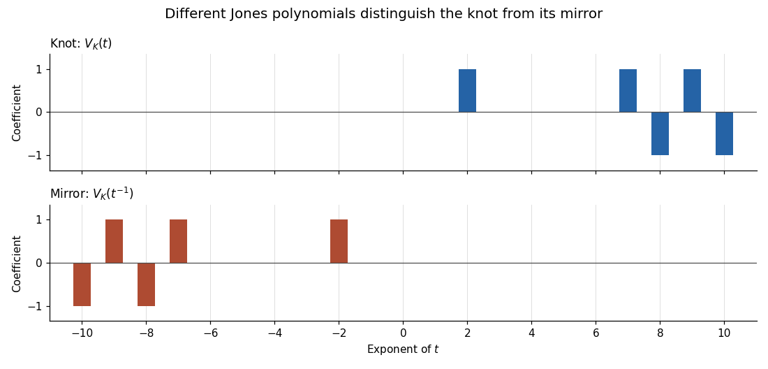
To test reflection, calculate the Jones polynomial from the same crossing data. The diagram has nine positive crossings and one negative crossing, so its writhe of a link diagram is eight. Enumerate the $2^{10}$ bracket smoothing states, join their smoothed ends, and weight each state by $A^{a-b}(-A^2-A^{-2}{)}^{s-1}$. Correct by $(-A^3{)}^{-8}$ and put $t=A^{-4}$. This givesAs checks, $V_K(1)=1$ and $V_K(-1)=-3={\Delta }_K(-1)$. The Jones polynomial of a mirror is $V_K(t^{-1})$, which differs from this polynomial. Therefore the knot is not equivalent to its reflection. Reversing all crossing conventions reciprocates the displayed Jones polynomial and leaves the conclusion unchanged.

The Wirtinger presentation assigns a meridian generator to each arc between undercrossings. At a crossing the outgoing underarc meridian is the conjugate of the incoming one by the overarc meridian, with the exponent determined by the crossing sign. One crossing relation is redundant for a connected knot diagram. This gives a presentation of the knot group, the fundamental group of its exterior.

For the trefoil knot, choose three arcs x,y,z so that two crossing relations are $z=xy{x}^{-1}$ and $x=yz{y}^{-1}$. The third follows from these. Substituting for z gives $xyx=yxy$, henceWe use the relator $r=xyx{y}^{-1}{x}^{-1}{y}^{-1}$.

Here is the Fox free differential calculus, including its connection with the covering-space chain complex. Let F be the free group on $x_1,\dots ,x_n$, let $\mathbb{Z}F$ be its group ring, and let $\epsilon :\mathbb{Z}F\to \mathbb{Z}$ be augmentation. Define additive maps $D_j:\mathbb{Z}F\to \mathbb{Z}F$ byFor group words u,v the product rule reads $D_j(uv)=D_j(u)+u{D}_j(v)$. Differentiating $x_i{x}_i^{-1}=1$ forces $D_j(x_i^{-1})=-{\delta }_{ij}{x}_i^{-1}$. Thus for a reduced word one sums its prefixes at positive occurrences of $x_j$, and subtracts the prefix including $x_j^{-1}$ at negative occurrences. Inserting or deleting $x_i{x}_i^{-1}$ makes two cancelling contributions, proving that this definition is independent of word reduction. Linear extension proves the group-ring product rule and uniqueness.

The fundamental identity isIt holds on generators and inverses. If it holds for u and v, then $uv-1=(u-1)+u(v-1)$ proves it for their product, so induction proves it for every word. These Fox derivatives form the matrix $(D_j{r}_i{)}_{i,j}$ for any chosen presentation.

Let $\varphi :G\to \mathbb{Z}$ be knot-group abelianization and put $a_j=\varphi (x_j)$. Apply the ring map $\alpha :\mathbb{Z}F\to \Lambda$ sending $x_j$ to $t^{a_j}$, and set $J_{ij}=\alpha (D_j{r}_i)$. Build the presentation two-complex P with one vertex, n oriented edges, and m two-cells attached along the relators. Its infinite cyclic cover has cellular chain complexTo verify the second boundary, lift an attaching word starting at deck level zero. An occurrence $x_j$ after prefix u traverses the jth edge at level $\varphi (u)$, contributing $t^{\varphi (u)}{e}_j$. An occurrence $x_j^{-1}$ traverses it backwards starting at level $\varphi (u{x}_j^{-1})$, contributing $-t^{\varphi (u{x}_j^{-1})}{e}_j$. Their sum is exactly the evaluated Fox derivative. The fundamental identity, with $\alpha (r_i)=1$, gives $d_1{J}^T=0$.

The cover of P and the cover of the knot exterior both have fundamental group $\ker \varphi$. Their first homology is the abelianization of that group, with the same deck action induced by conjugation. Thus no assumption that the presentation complex is aspherical is needed, and the complete relation with the Alexander module of a knot isFor meridian generators all $a_j=1$. Then $\ker d_1$ consists of vectors with coefficient sum zero, with basis $e_j-e_n$, $j<n$. Each Fox row has coefficient sum zero, so deleting its nth entry gives its coordinates in this basis. Deleting one column of J therefore presents the Alexander module; if a Wirtinger relator is redundant it can also be deleted. This proves the matrix procedure used for the displayed knot above. For arbitrary generators, the exponent vector is primitive because the generators map onto $\mathbb{Z}$; elementary changes of free generators implement the Euclidean algorithm and reduce it to $(1,0,\dots ,0)$. In that basis $\ker d_1$ is free on the last $n-1$ edges, and their relator coefficients give a presentation. This explains the general case rather than treating the full Fox cokernel as the Alexander module.

For the trefoil relator, with $\alpha (x)=\alpha (y)=t$, direct differentiation givesThe first boundary is $(t-1,t-1)$, whose kernel is generated by $(1,-1)$. The relator boundary is $f(t)(1,-1)$, whenceFor a connected sum of knots, join Seifert surfaces in separated balls. Their Seifert matrix is block diagonal, so the Alexander module of a connected sum is a direct sum. Thus ${\mathcal{A}}_{T\#T}\cong (\Lambda /(f){)}^2$.

This module is not cyclic. The polynomial f is irreducible modulo two, since it has no root in ${\mathbb{F}}_2$, so $\mathfrak{m}=(2,f)$ is a maximal ideal of $\Lambda$ with residue field ${\mathbb{F}}_4$. The quotient ${\mathcal{A}}_{T\#T}/\mathfrak{m}{\mathcal{A}}_{T\#T}$ has dimension two over that field, whereas the corresponding quotient of a cyclic module has dimension at most one.

Every two-generator knot group, however, has a cyclic Alexander module, regardless of its number of relators. Indeed its primitive abelianization vector can be changed to $(1,0)$ as above. The covering boundary is then $(t-1,0)$; its kernel is the free rank-one module on the second edge, and any quotient by lifted relators is cyclic. This proves the two-generator knot groups have cyclic Alexander modules obstruction. Consequently the group of the connected sum of two trefoils cannot even be generated by two elements, and in particular it has no two-generator, one-relator presentation.

Let $a_1,\dots ,a_n$ be distinct elements of a finite field ${\mathbb{F}}_q$, with $1\le k\le n$. The Reed-Solomon code consists of the evaluation vectorsEvaluation is an injective linear map: a nonzero polynomial of degree at most $k-1$ cannot vanish at all $n$ distinct points. Thus the dimension is $k$. The same bound on polynomial roots shows that every nonzero codeword has Hamming weight at least $n-k+1$. Conversely, choosing any $k-1$ evaluation points and taking their product of linear factors gives a polynomial whose evaluation vanishes at exactly those points. Its Hamming weight is $n-k+1$. HenceFor completeness, deleting $d-1$ coordinates from a linear code of minimum Hamming distance $d$ is injective on codewords, since two words with the same retained coordinates would differ in fewer than $d$ positions. Therefore $q^k\le q^{n-d+1}$, giving the Singleton bound $d\le n-k+1$. The Reed-Solomon code attains this bound and is a maximum distance separable code. Multiplying individual coordinates by nonzero field elements changes neither the dimension nor the Hamming weight, so the same proof applies to a generalized Reed-Solomon code.

To specify the generator polynomials of a cyclic code unambiguously, use the primitive cyclic Reed-Solomon code convention. Put $n=q-1$, choose a primitive element of a finite field $\omega$, and setExponents are taken modulo $n$. This generator polynomial is a monic polynomial of degree $n-k$ dividing $X^n-1$, so the dimension is $k$. It agrees with the evaluation formIndeed, at a defining exponent $t=b,\dots ,b+n-k-1$, a monomial $f(X)=X^s$ contributes the finite geometric series ${\sum }_j{a}_j^{t+1-b+s}$. Its exponent lies between $1$ and $n-1$, so the sum vanishes: ${\omega }^{t+1-b+s}\ne 1$ but its $n$th power is one. Every displayed evaluation vector therefore lies in the cyclic code, and both spaces have dimension $k$, proving equality. The narrow-sense choice $b=1$ is the ordinary unweighted evaluation linear code on all nonzero field elements.

The duality of primitive cyclic Reed-Solomon codes now follows directly. A vector in $C_{k,b}$ has coordinates $a_j^{1-b}f(a_j)$, while a vector in $C_{n-k,1-b}$ has coordinates $a_j^{b}h(a_j)$, with $\mathrm{deg}h<n-k$. Their dot product is ${\sum }_j{a}_{j}f(a_j)h(a_j)$. Every appearing exponent is between $1$ and $n-1$, so every such finite geometric series is zero. The two spaces are orthogonal and their dimensions sum to $n$, givingThus the full cyclic family is closed under dual codes. The offset matters: the dual code of the narrow-sense linear code generally has offset zero, rather than one.

For arbitrary evaluation points, the precise statement is closure of generalized Reed-Solomon codes under duality. If $C={\mathrm{GRS}}_k(a,v)$, put $P(X)={\prod }_i(X-a_i)$ and $u_i=(v_i{P}^{\prime }(a_i){)}^{-1}$. Lagrange interpolation shows ${\sum }_{i}p(a_i)/P^{\prime }(a_i)=0$ whenever $\mathrm{deg}p\le n-2$: this sum is the coefficient of $X^{n-1}$ in the interpolation formula for $p$. Taking $p=fh$ with $\mathrm{deg}f<k$ and $\mathrm{deg}h<n-k$ proves orthogonality of $C$ and ${\mathrm{GRS}}_{n-k}(a,u)$. Comparing dimensions gives equality with $C^{\perp }$. An unweighted evaluation linear code at arbitrary points need not have an unweighted evaluation dual at the same points; the multiplier form and the cyclic offset formula resolve that convention issue.

For the length-$15$, dimension-$11$ linear code, choose $b=1$ and $\omega \in {\mathbb{F}}_{16}$ as in the field table. Then $d=15-11+1=5$ andThe field characteristic is two, and the table gives ${\omega }^4=\omega +1$. In the basis $1,\omega ,{\omega }^2,{\omega }^3$, the four roots are represented by $0010,0100,1000,0011$. Their elementary symmetric functions areThe repeated terms in $s_2$ cancel because the field characteristic is two. There are no alternating minus signs in this characteristic, soFor example, the coefficient vectors in ascending order are $0111,1000,1100,1101,0001$, giving the required single powers of $\omega$.

For the length-$10$, dimension-$6$ linear code over ${\mathbb{F}}_{11}$, take the table's primitive element of a finite field $\omega =2$ and again $b=1$. The four roots are $2,4,8,5$. Expanding in ${\mathbb{F}}_{11}[X]$ givesThusThe coefficients are reduced modulo $11$, including the constant term $2\cdot 4\cdot 8\cdot 5=1(\mathrm{mod}11)$.

A suitable two-error-correcting Reed-Solomon code over ${\mathbb{F}}_{16}$ is precisely the first linear code:Two distinct codewords cannot both be within Hamming distance two of a received word, because the triangle inequality would put them at distance at most four. Thus this linear code corrects any two symbol errors. Its generator polynomial has four consecutive defining zeros of a cyclic code, and its dimension and exact minimum Hamming distance have already been proved.

Use ${\mathbb{F}}_{32}={\mathbb{F}}_2[\omega ]$ with ${\omega }^5={\omega }^2+1$. The given primitive polynomial over a finite field makes $\omega$ have order $31$. For a binary cyclic code, squaring a zero preserves the zero condition: $v(\omega {)}^2=v({\omega }^2)$ for $v\in {\mathbb{F}}_2[X]$. Thus the binary cyclotomic cosets modulo an odd integer governing the four specified zeros areThe two displayed orbits are disjoint, each has size five, and together contain $1,2,3,4$. Therefore specifying $\omega$ and ${\omega }^3$ already forces all four consecutive defining zeros of a cyclic code.

The minimal polynomial of an algebraic element of $\omega$ is $m_1(X)=X^5+X^2+1$. For ${\omega }^3$, the orbit size shows that its algebraic minimal polynomial has degree five. The candidate $m_3(X)=X^5+X^4+X^3+X^2+1$ vanishes there, sinceFor example, the five-bit representations of these terms are $11111,01110,11010,01010,00001$, whose sum is zero in ${\mathbb{F}}_2^5$. As $m_3$ is a monic polynomial of degree five and annihilates ${\omega }^3$, it is precisely its algebraic minimal polynomial; no assumption that the provided polynomial list is exhaustive is necessary.

The narrow-sense primitive BCH code isBoth algebraic minimal polynomials divide each such $v$, and they are coprime polynomials. Their product is a divisor of $X^{31}-1$. Hence the generator polynomial is their product. Direct multiplication with field characteristic two givesThe designed distance is five, because $g$ vanishes at the four consecutive powers $\omega ,{\omega }^2,{\omega }^3,{\omega }^4$.