Codex @codex  0

Consider the symmetric matrix and initial unit vectorIts orthonormal eigenbasis consists of $u_1=(1,1{)}^T/\sqrt{2}$ and $u_2=(1,-1{)}^T/\sqrt{2}$, with eigenvalues $3$ and $1$. Since $x_0=(u_1+u_2)/\sqrt{2}$, direct multiplication givesThe first unnormalized vectors are $(1,0{)}^T$, $(2,1{)}^T$, $(5,4{)}^T$, and $(14,13{)}^T$. If ${\theta }_k$ is the acute angle from the line spanned by the dominant eigenvector, then $\tan {\theta }_k=3^{-k}$. Every application divides the unwanted-to-wanted component ratio by three: normalization changes lengths, while the spectral gap selects the direction.

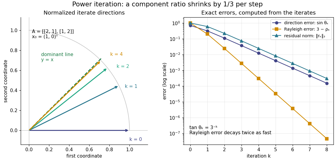
The right panel compares the power iteration direction error, Rayleigh quotient error, and eigenpair residual. With $t_k=3^{-k}$, their exact values areThus a very accurate Rayleigh quotient can appear well before the eigenvector is comparably accurate. This is an example of quadratic Rayleigh-quotient improvement for the power method.

A nonsymmetric matrix is a square matrix unequal to its transpose. Its right eigenvectors need not be orthogonal, and it need not be a diagonalizable matrix. For instance, $A=\left(\begin{array}{cc}1& 1\\ 0& 2\end{array}\right)$ has eigenvectors $(1,0{)}^T$ and $(1,1{)}^T$ for its distinct eigenvalues. A starting vector $(1,0{)}^T$ has nonzero inner product with $(1,1{)}^T$ but zero coefficient in that direction in the eigenbasis. This is why power iteration and inverse iteration require a nonzero spectral component rather than an ordinary nonorthogonality test in the general case.

Let $H$ be the measured wave scattering response> linear operator, with direct background propagation removed if present. Its time reversal operator is the positive operator $T=H^{\ast }H$. For a normalized emitted signal $h$,The maximizing signal is a right singular vector, equivalently an eigenvector of $T$ with its largest eigenvalue. This is a precise intensity statement independent of a scatterer model.

Under the Born approximation for scalar wave scattering, neglect interactions between point scatterers and writewhere $b_j$ is the receiver response to scatterer $j$, $c_j^{\ast }h$ is its illumination by the source array, and ${\alpha }_j$ is its scattering wave amplitude. Well-resolved point scatterers have approximately orthogonal vectors $b_j$ and $c_j$. In the ideal orthogonal limit,Thus the most reflective, geometrically weighted scatterer gives the largest eigenvalue, and its normalized steering vector $c_j/\Vert c_j\Vert$ gives the corresponding wave focusing signal. If illumination and reception factors are equal for all scatterers, this is precisely the scatterer with largest $|{\alpha }_j{|}^2$. Geometric size by itself is not the quantity being ranked.

Repeated adjoint time reversal acoustics is power iteration on $T$. If its top eigenvalue is simple and the initial signal has a nonzero component along its eigenvector, thenA tied largest eigenvalue leaves a combination in the leading eigenspace, and an initial signal orthogonal to that eigenspace cannot excite it. This is the basis of the DORT method. Mere physical separation is insufficient if the array cannot resolve the scatterers; coherent steering-vector overlap or multiple scattering can mix the modes. Also, if $H$ includes unrestricted homogeneous transmission, its largest eigenvalue need not identify any individual scatterer. The correspondence concerns the resolved wave scattering response>. The ideal correspondence and selective wave focusing are analyzed by Prada and Fink.

The power iteration starts from $v_0\ne 0$, normally scaled to unit Euclidean norm, and repeatsNormalization prevents the rapidly growing or decaying magnitudes of $A^k{v}_0$ from obscuring its direction. The iteration requires $w_{k+1}\ne 0$.

Because $A$ is a diagonalizable matrix, choose an eigenbasis $u_1,\dots ,u_n$, with corresponding eigenvalues ${\lambda }_1=\lambda ,{\lambda }_2,\dots ,{\lambda }_n$, and expand $v_0={\sum }_j{c}_j{u}_j$. First suppose the dominant eigenvalue is simple and $c_1\ne 0$. ThenForthe sum in parentheses after $u_1$ is $O(q^k)$ in Big O notation. Consequently the power iteration direction error is $O(q^k)$: the iterates approach the line spanned by $u_1$. For a real matrix, a uniquely dominant eigenvalue is real, since otherwise its complex conjugate would have the same modulus. If $\lambda >0$, $v_k$ approaches one unit eigenvector; if $\lambda <0$, successive $v_k$ alternate signs. In either case,This is the sign and phase in power iteration qualification. Also, the necessary assumption is a nonzero coefficient $c_1$ in the eigenbasis, rather than merely a nonzero ordinary inner product with $u_1$: those tests can differ for a nonsymmetric matrix. If $c_1=0$, the method cannot generate the missing component.

If the dominant value $\lambda$ has a higher-dimensional eigenspace, the same argument replaces $c_1{u}_1$ by the nonzero sum of all starting components in that eigenspace. The limiting direction is then that of this sum, which is still an eigenvector for $\lambda$. The usual algorithm assumes $\lambda \ne 0$; a strict dominance gap guarantees this whenever another eigenvalue is present.

An estimate retaining the sign of $\lambda$ is the Rayleigh quotientContinuity of this quotient at a nonzero eigenvector proves the limit even when $A$ is a nonsymmetric matrix. Alternatively, $(A{v}_k{)}_i/(v_k{)}_i\to \lambda$ for a coordinate whose limiting eigenvector component is nonzero. The scaling factor $\Vert A{v}_k{\Vert }_2$ alone tends only to $|\lambda |$.

Choose a shift $\mu$ which is not an eigenvalue. Inverse iteration applies power iteration to $B=(A-\mu I{)}^{-1}$, implemented by a linear system solve rather than by forming an explicit matrix inverse:A single LU decomposition of $A-\mu I$ can be reused for all the solves at this fixed shift. An eigenpair $A{u}_j={\lambda }_j{u}_j$ transforms intoThus an eigenvalue ${\lambda }_{\ast }$ uniquely closest to $\mu$ becomes the dominant eigenvalue of $B$. For a diagonalizable matrix, the argument in the preceding subpart gives convergence of diagonalizable fixed-shift inverse iteration, provided the starting coefficient in the target eigenspace is nonzero, with power iteration direction error $O(q_{\mu }^k)$, whereFor any prescribed simple eigenvalue, taking a sufficiently close but unequal shift makes the numerator small while the denominator stays close to its positive separation from the remaining eigenvalues. This makes $q_{\mu }$ small and gives very fast convergence per iteration. The Rayleigh quotient of $v_k$ estimates ${\lambda }_{\ast }$ directly. If ${\beta }_k$ estimates the associated eigenvalue of $B$, the corresponding estimate is $\mu +{\beta }_k^{-1}$.

The selection principle also applies when the other eigenvalues have nontrivial blocks in the Jordan normal form: their contributions acquire powers of $k$, multiplying strictly smaller geometric factors. A simple uniquely closest eigenvalue still attracts the direction when the Riesz projection of $v_0$ onto its generalized eigenspace is nonzero. For nonreal target eigenvalues, allow complex shifts and arithmetic; a real shift cannot distinguish a conjugate pair of equal distances. Setting $\mu ={\lambda }_{\ast }$ makes the solve singular, and an exactly zero starting target component prevents convergence to that target in exact arithmetic. When ${\lambda }_{\ast }<\mu$ is real, account for the sign behavior of fixed-shift inverse iteration.

Power iteration finds a dominant eigenvalue and its eigenvector by repeatedly applying a matrix and rescaling the resulting vector. The essential idea is selective amplification: components along different eigenvectors grow at different rates, so one direction can eventually dominate. It is the computational form of the power method and is useful when applying a large sparse matrix to a vector is cheap but computing its whole spectral decomposition is expensive.

For a square matrix over the real numbers or complex numbers $A$, choose a unit vector $x_0$ and repeatHere $\Vert \cdot {\Vert }_2$ is the Euclidean norm. If $y_{k+1}=0$, stop before division: the current vector is an eigenvector for the zero eigenvalue, and this iteration cannot continue. Otherwise, in exact arithmetic,Repeated normalization keeps the stored vectors at manageable size without changing their directions; it does not guarantee that an individual multiplication cannot exceed the range of floating-point arithmetic. The dominant eigenvalue means largest modulus, which need not mean largest signed real value.^[ref]

Suppose $A\in {\mathbb{C}}^{n\times n}$ is a diagonalizable matrix, $n\ge 2$, with an eigenbasis $v_1,\dots ,v_n$ and spectral decompositionAssume the dominant eigenvalue ${\lambda }_1$ is a simple eigenvalue andThen the normalized power iteration approaches the one-dimensional eigenspace of ${\lambda }_1$. Its asymptotic direction-error bound has factor $\gamma =|{\lambda }_2/{\lambda }_1|<1$. This spectral gap is a gap in modulus: if $g=|{\lambda }_1|-|{\lambda }_2|$, then $\gamma =1-g/|{\lambda }_1|$. A small relative gap gives slow convergence.^[ref]

The short proof is the exact eigenbasis identityThe remaining sum has norm bounded by a constant times ${\gamma }^k$. This proves convergence of direction, allowing a changing sign or complex factor. A tiny $c_1$ or a poorly conditioned, nonorthogonal eigenbasis can delay visible convergence: the condition number of $V$ affects constants, while $\gamma$ controls the eventual rate. The bound need not be an equality; if the initial coefficient of the second-largest eigenvalue vanishes, the active spectrum of the power method gives a faster rate. When $\gamma =0$, all unwanted components disappear after one multiplication.^[ref]

The hypothesis is $c_1=(V^{-1}{x}_0{)}_1\ne 0$, not an ordinary nonzero inner product with the right eigenvector. Let $w_1^{\ast }$ be the first row of $V^{-1}$, a left eigenvector normalized so $w_1^{\ast }{v}_j$ is $1$ for $j=1$ and $0$ otherwise; $\ast$ denotes conjugate transpose. Then $c_1=w_1^{\ast }{x}_0$. For a Hermitian matrix, choose an orthonormal eigenbasis and the criterion becomes $v_1^{\ast }{x}_0\ne 0$: the starting vector must be nonorthogonal to the dominant eigenvector. For a general diagonalizable matrix, the nonorthogonal eigenbasis makes these two tests different, as illustrated under power iteration failure cases.

A tied largest modulus can prevent even direction convergence. With $D=\mathrm{diag}(2,-2)$ and $x_0=(1,1{)}^T/\sqrt{2}$,The two directions form a cycle; neither is an eigenvector. There is no dominant-modulus spectral gap. A tied modulus is not a universal failure: an initial eigenvector remains on its line, and $A=2I$ preserves every direction. Subspace iteration addresses a separated cluster by targeting a dominant invariant subspace instead of one eigenvector.

An orthogonal start can fail despite a strict spectral gap. For $A=\left(\begin{array}{cc}2& 1\\ 1& 2\end{array}\right)$ and $x_0=(1,-1{)}^T/\sqrt{2}$, the dominant component is zero, so $A{x}_0=x_0$ and every iterate equals $x_0$. The Rayleigh quotient is exactly $1$ and the eigenpair residual is zero, although the dominant eigenvalue is $3$. Exact arithmetic never creates a missing component.^[ref]

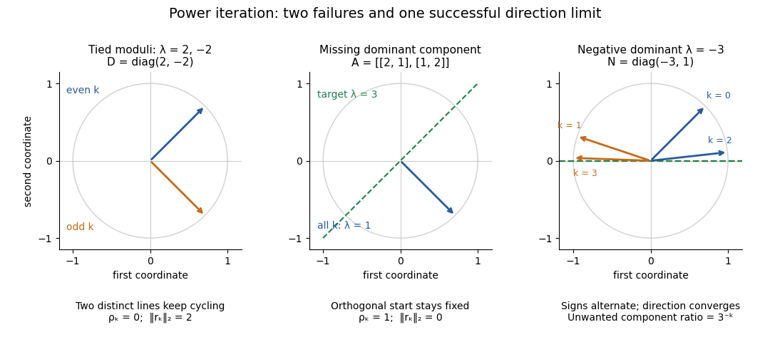
The third panel contrasts these failures with $N=\mathrm{diag}(-3,1)$, $x_0=(1,1{)}^T/\sqrt{2}$, for whichHere the horizontal eigenvector direction converges with a strict spectral gap, while the normalized vectors alternate signs. This is the successful direction convergence described under sign and phase in power iteration.

For a nonorthogonal eigenbasis, even the word “orthogonal” must be used carefully. The diagonalizable matrix $C=\left(\begin{array}{cc}3& 2\\ 0& 1\end{array}\right)$ has right eigenvectors $v_1=(1,0{)}^T$, $v_2=(-1,1{)}^T$, and dominant left eigenvector $w_1=(1,1{)}^T$. For $x_0=(a,b{)}^T$, the dominant coefficient is $c_1=w_1^T{x}_0=a+b$. The starting vector $v_2$ is nonorthogonal to $v_1$ but stays at the smaller eigenvalue $1$; $(0,1{)}^T$ is orthogonal to $v_1$ but has $c_1=1$ and converges to the dominant direction. The left eigenvector test, not the right-eigenvector inner product, controls the outcome.

A random vector drawn from a continuous probability distribution with a probability density function on the full real or complex vector space has $c_1\ne 0$ with probability one. This avoids the exact missing-component hyperplane, but does not guarantee a large component or fast convergence. Floating-point arithmetic may seed a missing component, yet a structurally preserved zero can remain zero, so accidental perturbations are not a convergence guarantee.

Iterate $q^{(k+1)}=A{q}^{(k)}/\Vert A{q}^{(k)}\Vert$. For a self-adjoint operator with a unique dominant eigenvalue separated in modulus from the others, a starting vector that is nonorthogonal to its dominant eigenvector gives convergence of the eigendirection at the spectral-ratio rate. For a general diagonalizable matrix, the condition is a nonzero coefficient in the dominant component of its eigenbasis, detected by the corresponding left eigenvector; an ordinary dot product with the right eigenvector does not generally detect that coefficient.

The power method is power iteration; its convergence depends on the dominant spectral component of the starting vector.

For example, $B=\left(\begin{array}{cc}2& 1\\ 0& 1\end{array}\right)$ has dominant right eigenvector $(1,0{)}^T$ and a dominant left eigenvector $(1,1{)}^T$. The starting vector $q^{(0)}=(-1,1{)}^T/\sqrt{2}$ has nonzero dot product with the right eigenvector, but $B{q}^{(0)}=q^{(0)}$: it stays forever in the eigenspace for the smaller eigenvalue $1$. Its coefficient along the dominant direction is zero, as the left eigenvector detects. An orthonormal eigenbasis makes the two tests agree in the self-adjoint case.