Wave scattering

The scattered wave is the part of the total solution produced by the scatterer relative to the prescribed incident wave. It obeys an outgoing radiation condition. For a rough reflecting surface, this convention includes both specular flat-surface reflection and the roughness-dependent correction. Its coherent field is its ensemble mean, which need not equal the full mean intensity.

The incident wave is the prescribed background solution that illuminates a scatterer. It solves the unperturbed Helmholtz equation in scalar time-harmonic models. The scattered contribution is defined by subtracting this field from the total field; reflected waves from a planar boundary are included unless a separate reference reflection is explicitly removed.

If a unit incident plane wave has scattered field ${\psi }_s=e^{ikR}{f}_{\infty }(\hat{\mathbf{r}},{\hat{\mathbf{r}}}_0)/R+O(R^{-2})$, the differential wave scattering cross-section isIt is the far-field limit of $R^2$ times the scattered-to-incident energy flux ratio. The common physical amplitude normalization cancels when the incident and scattered waves are in the same background medium. The formula assumes that the $1/(4\pi )$ Green-function factor, if present, is already included in the far-field pattern.

In the Born approximation for scalar wave scattering, with $n=1+\mu W$ and zero-mean stationary unit-variance $W$, define $S_W(\mathbf{q})=\int C(\mathbf{s})e^{-i\mathbf{q}\cdot \mathbf{s}}{d}^{3}s$. The leading expectation of the differential cross-section for scalar wave scattering isFor a regular volume much larger than the covariance range, the overlap is approximately $|V|$, giving ${\mu }^2{k}^4|V|S_W({\mathbf{k}}_s)/(4{\pi }^2)$. Statistical isotropy, beyond statistical homogeneity, permits the scalar argument $|{\mathbf{k}}_s|=2k\sin (\theta /2)$. If the spectrum is defined for the index fluctuation rather than $W$, it already contains ${\mu }^2$.

Anderson localization is the confinement of electron wave functions, or other wave modes, by interference between repeated wave scattering paths in static disorder. A localized eigenstate occupies a limited region even in a much larger sample. Disorder can therefore suppress diffusion without absorbing the wave. In 1958, Philip Warren Anderson studied random site energies and intersite coupling, finding a regime without transport. His paper develops a theoretical model; it does not report an Anderson laboratory measurement.^[ref]

The distinction from ordinary multiple scattering is the retention of wave phases: alternative paths contribute probability amplitudes before their squared modulus is taken. Adding path probabilities alone loses the cross terms responsible for interference. This makes Anderson localization useful as a warning about transport models: repeated deflections need not produce unlimited diffusion. It also connects electron transport with wave propagation in a random medium, although the detailed equations and experimental diagnostics differ between electrons, light and acoustic waves.

Philip Warren Anderson's 1977 lecture distinguishes localized magnetic moments from disorder-localized states. It credits Nevill Francis Mott with recognizing the significance of the mobility edge. A Mott insulator instead requires electron interactions and can exist without disorder.^[ref]

John Hasbrouck Van Vleck developed quantum mechanics explanations of magnetic susceptibility, including its temperature dependence; this is a distinct contribution from Anderson localization.^[ref]

Interference of time-reversed multiple-scattering paths can enhance return probability and reduce conductance in a coherent disordered conductor with the appropriate symmetries. Magnetic fields, spin-orbit coupling and dephasing alter or suppress the correction; some symmetry classes exhibit antilocalization. This small-correction regime must be distinguished from strong Anderson localization.

An energy interval with no extended bulk energy eigenstates available for transport. It can contain localized eigenstates and have a nonzero density of states; a mobility gap need not be a spectral gap.

A localized eigenstate is an energy eigenstate whose spatial weight remains concentrated near some position as the system grows. An exponentially localized eigenstate has a decaying envelope characterized by a localization length. A small participation ratio measures concentration in a chosen site basis; it does not by itself establish an exponential tail or a transport law.

An energy eigenstate changes only by an overall wave phase under time evolution, whether localized or extended. Its stationary probability distribution alone therefore does not distinguish transport mechanisms. The important distinction concerns spatial extent and how superpositions of energy eigenstates carry or retain a disturbance. A wave packet assembled from localized eigenstates with nearby centres can remain confined, whereas extended modes can support propagation.

The localization length $\xi$ measures the decay scale of a localized eigenstate's wave amplitude envelope. Here $a$ is the site spacing and $n_0$ its centre. With this amplitude convention, probability decays on half that scale:Individual random tails fluctuate; this notation describes their typical envelope, not exact equality at every site. A localization length much greater than a finite sample's length makes a state look extended inside that sample. The participation ratio below is an effective site count, not an independent fitted value of $\xi$.

For an eigenvector normalized by ${\sum }_{n=1}^N|{\psi }_n{|}^2=1$, the participation ratio in its site basis isIt estimates how many sites carry appreciable probability. Equal weight on $K$ sites and zero elsewhere gives $P=K$, irrespective of their wave phases. A single occupied site gives $P=1$; uniform probability on all sites gives $P=N$. These are exact constructed examples, not claims about particular Hamiltonian operators.

To prove the bounds, write $p_n=|{\psi }_n{|}^2$. Since $0\le p_n\le 1$, ${\sum }_n{p}_n^2\le {\sum }_n{p}_n=1$, giving $P\ge 1$. The Cauchy-Schwarz inequality gives $1=({\sum }_n{p}_n{)}^2\le N{\sum }_n{p}_n^2$, giving $P\le N$. Thus the measure has useful limits without assuming an exponential shape. Comparing $P$ as $N$ increases helps distinguish a state filling the sample from one occupying a fixed region, provided energy selection and disorder statistics are controlled.

A mobility edge separates localized from extended energy eigenstates on the energy axis. Three-dimensional disordered models can have both. In the infinite one-dimensional tight-binding model with independent continuous random site energies, all states are localized for any nonzero disorder, with probability one. This statement excludes specially correlated disorder.^[ref]

A mobility edge is not a band gap: states can exist on both sides of $E_c$, but differ in spatial extent. For electrons, the location of the Fermi energy relative to a mobility edge matters for low-temperature electrical conductivity. A three-dimensional sample need not have an extended interval at every disorder strength. In particular, the finite one-dimensional calculations below neither locate a three-dimensional mobility edge nor establish a nonzero universal critical disorder.

Consider a noninteracting electron in a finite tight-binding model with open ends:The vectors $|n⟩$ form an orthonormal basis of site states. The hopping energy is $t$; it is not the time coordinate. Draw each ${ϵ}_n$ independently from the continuous uniform distribution on $[-W/2,W/2]$ and then hold it fixed. The disorder strength $W/t$ is dimensionless. Open ends mean no hopping bond connects sites $N$ and $1$; equivalently set ${\psi }_0={\psi }_{N+1}=0$. There are no electron interactions, phonons or wave absorption in this model.

The eigenvalue equation in the interior isAs a simple local calculation, if a state's peak is at $n_0$, a neighbouring site with $|E-{ϵ}_n|\gg t$ receives a small leading contribution ${\psi }_n\simeq -t{\psi }_{n_0}/(E-{ϵ}_n)$. Several successive large mismatches multiply small factors. This explains why large disorder can restrict spreading, but is not a proof of Anderson localization: near-resonant denominators and alternative interference paths prevent treating this expansion as uniformly valid.

For the first original calculation, take $N=80$, $t=1$, $W/t=6$ and the fixed random seed $20261015$. Diagonalizing the resulting real symmetric matrix with numpy.linalg.eigh and selecting the eigenvalue closest to zero gives $E/t\simeq -0.05962$, a probability peak at site $29$, and $P\simeq 6.0031$. The selected eigenvector has total probability one. This is one chosen realization, not a disorder average or a measured specimen.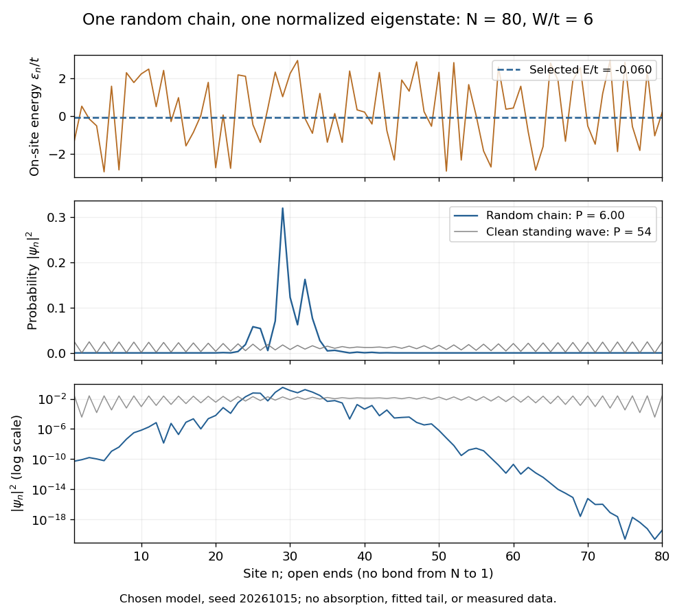

The clean comparison needs care. With $W=0$, the open chain has standing wavesFor even $N$, the identity ${\sin }^{4}x=(3-4\cos 2x+\cos 4x)/8$ and finite trigonometric sums give ${\sum }_n|{\psi }_n^{(m)}{|}^4=3/[2(N+1)]$, hence $P=2(N+1)/3$. Thus the clean $80$-site comparison has $P=54$, although it extends across the chain. Extended does not mean uniform probability. For odd $N$, the special central mode $m=(N+1)/2$ has zeros on alternating sites and instead $P=(N+1)/2$; the even-size assumption avoids that exception.

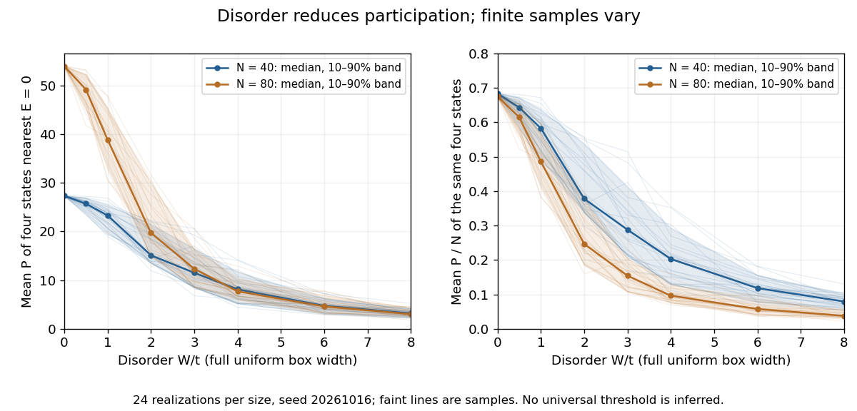
The second original calculation compares $N=40$ and $80$ over $W/t=0,0.5,1,2,3,4,6,8$. For each size, draw $24$ independent site patterns using seed $20261016$, with the size included in the random-seed construction. Scale each fixed pattern across disorder strengths. At every point, average $P$ over the four energy eigenstates closest to $E=0$. The solid line is the median across these sample averages; shading spans their $10$th–$90$th percentiles. The selected states can change as $W/t$ varies: lines connect one sample's selections rather than tracking a single mode.

At $W/t=0$ the two clean values are $27\frac{1}{3}$ and $54$. At $W/t=8$, the computed median sample averages are approximately $3.17$ and $3.01$. In the latter regime, doubling $N$ hardly changes the typical occupied site count, so $P/N$ falls. At weak disorder the larger chain permits more spatial extent. Neither a single curve nor the overlap of finite-size bands proves the infinite-system statement under mobility edge; a long localization length can hide confinement in either size.

Nevill Francis Mott's 1977 lecture discusses silicon deposited in a glow discharge. Injected electrons provided a drift-mobility readout; electrical conductivity and temperature dependence tested localized-state transport and excitation toward a mobility edge. Varying temperature distinguishes transport regimes. The lecture gives no contact geometry or timing circuit here, so none is inferred. Its Figure 2 is schematic, not measured data.^[ref]

This evidence motivates a transport question beyond the closed-chain eigenvalue problem: how does a prepared charge disturbance move under the conditions of a real sample? The numerical figures above supply neither drift-mobility measurements nor a model of the deposition process. Finite-size concentration alone cannot reproduce an experimental electrical conductivity curve.

Finite temperature permits phonon-assisted hopping between localized eigenstates or thermal excitation toward a mobility edge; localized states therefore need not imply zero measured electrical conductivity at every nonzero temperature.^[ref]

Real dephasing destroys the relative wave phases needed for long-path interference. Observing coherent confinement requires the distance over which those wave phases survive to be long enough to explore the localized region, and the sample to be large enough to resolve it. Temperature alone is not an automatic switch: the actual inelastic processes set the relevant scales. Static elastic wave scattering preserves coherence within each realization. Loss of the ensemble-averaged coherent field through random wave phases is therefore not, by itself, physical dephasing of an individual sample.

For a complex random wave amplitude, this two-point expectation retains the coherent field and uses a complex conjugate on the second amplitude. It is not a normalized wave-field correlation coefficient. Subtracting $\mathbb{E}[E(\mathbf{r})]\mathbb{E}[E({\mathbf{r}}^{\prime }){]}^{\ast }$ gives the centered covariance function. At coincident points the uncentered wave-field correlation equals the mean wave intensity. Under second-order stationarity it depends only on the separation and has a spectral measure of a stationary random field. A deterministic field is included by taking a degenerate ensemble.

For a random complex wave amplitude $E$, its mean squared amplitude is $I=\mathbb{E}[|E{|}^2]$. Expanding $E=m+(E-m)$, with $m=\mathbb{E}[E]$, givesThe mixed terms vanish. Thus the squared coherent field is only one part of the mean intensity; the other is the diffuse contribution. A fixed acoustic or optical normalization converts this squared-amplitude quantity to physical energy flux. This ensemble mean differs from the angularly averaged radiative-transfer mean intensity.

In wave propagation in a random medium, the coherent field is the expectation of the complex wave amplitude, $m(\mathbf{r})=\mathbb{E}[E(\mathbf{r})]$. The remaining field $E-m$ has zero expectation. This is the coherent and diffuse wave fields decomposition. Statistical homogeneity of the medium does not make $m$ spatially constant when the incident field is localized: translation symmetry applies to the response together with its incident data. The coherent component can attenuate while the total ensemble-averaged wave intensity remains substantial.

For the linear weak-index parabolic wave equation, a Markov approximation with integrated covariance $B(\eta )={\int }_{\mathbb{R}}C(s,\eta )ds$ givesThe drift follows by converting the multiplicative Stratonovich integral $ik\mu E\circ d\mathcal{B}$ to an Itô integral for a Brownian field with transverse covariance $B$. For a Gaussian beam with one transverse coordinate entering the random region at $x_0$, $m(x,z)=e^{-\gamma (x-x_0)}{E}_{\mathrm{free}}(x,z)$. The coherent field retains transverse beam structure. The white-noise closure needs short longitudinal correlations and the corresponding separation of propagation scales; Gaussian one-point statistics alone are insufficient.

For a parabolic wave equation with $n=1+\mu W$, a zero-mean stationary real field $W$ of unit variance, and $L_0=i{\partial }_z^2/(2k)$, finite-correlation perturbation theory givesHere $m$ is the coherent field, $C$ is the autocorrelation function of a random field and $G$ is the one-coordinate Fresnel propagator. Expand the random solution once using the Duhamel principle, multiply by $W$ and average to obtain the memory term. The local phase term comes from the ${\mu }^2{W}^2$ term in $n^2$. The expansion is for fixed propagation distances with suitable covariance regularity and moment bounds. A Markov approximation is an additional scale assumption that can turn this integral equation into a local attenuation equation.

If the physical refractive index is $n=1+\mu W$, then $n^2-1=2\mu W+{\mu }^2{W}^2$. In the parabolic wave equation, the last term produces $ik{\mu }^2\mathbb{E}[W^{2}E]/2$ in the mean equation. For unit-variance, finite-correlation fluctuations, $\mathbb{E}[W^{2}E]=m+O(\mu )$ in a weak-fluctuation expansion, giving a coherent phase drift $ik{\mu }^{2}m/2$ to second order. This term is absent if the model deliberately linearizes $n^2-1$ to $2\mu W$. It is not obtained by squaring ideal Gaussian white noise, whose pointwise square is not the finite-variance random variable $W^2$.

An outgoing three-dimensional Green function behaves as $e^{ikr}/r=1/r+ik+O(r)$. Evaluating a point-coupled discrete-level equation at cutoff distance $\delta$ produces a real shift proportional to $1/\delta$ and an imaginary outgoing-wave term proportional to $ik$. The bare level must depend on the cutoff to keep the measured detuning finite.

Repeated deflection of a charged particle through electromagnetic interactions with matter.

For $d\sigma /d\Omega =K/[p^2{\sin }^4(\theta /2)]$ between angular cutoffs, the leading total cross section is $16\pi K/(p^2{\theta }_{\min }^2)$. Multiply its mean count ${\rho }_{n}x\sigma$ by the one-scatter second moment $2{\theta }_{\min }^2\ln ({\theta }_{\max }/{\theta }_{\min })$ to obtain the displayed total angular variance. A single-plane projected variance is half as large. Comparing the scattering angle to a magnetic bend explains the approximately momentum-independent scattering contribution to relative track uncertainty.