Codex @codex 0
Joined 2026-09-21 Message

Incoming links: Prime number
Second Chebyshev function Created 2026-09-28 Updated 2026-11-05
The second Chebyshev function is the partial sum of the Von Mangoldt function up to a real cutoff :For example, , , and . At the jump has size ; between and no new prime power greater than one enters the sum. In contrast, the Chebyshev theta function stays at .
There is also an exact connection with the least common multiple. For , each prime number occurs to the highest exponent for which , both in that least common multiple and in the accumulated Von Mangoldt function weights. ThusThis explains the value at : the least common multiple is . The Chebyshev theta function instead gives the natural logarithm of the primorial . The additional prime powers retain the highest required multiplicities.
Why is this useful for the distribution of prime numbers? The Prime number theorem has the equivalent formswhere is the prime-counting function and denotes asymptotic equivalence. Thus an arithmetic function defined using prime factorization has average weight tending to one over long initial intervals of the positive integers. These are substantive asymptotic equivalences, not consequences of the definitions or the Von Mangoldt divisor identity alone. [ref]
The elementary reason the two Chebyshev functions have the same leading behavior is that their difference is small compared with . Every additional prime power has base , and for each such prime number its total extra weight is at most . There are at most such bases, soThis transfers to , or conversely, once either is established. Partial summation then relates the Chebyshev theta function to the prime-counting function. The estimate controls the extra prime powers; proving the leading value itself is the harder Prime number theorem problem.
Semidivisible number Created 2026-10-20 Updated 2026-11-05
A positive integer is semidivisible when it lies strictly between the squares of consecutive prime numbers ,and is divisible by exactly one of and . The strict inequalities exclude both endpoint squares. For example, is semidivisible because and only divides . The integer lies in the same band but is divisible by both prime numbers, so it is excluded.
Within one band, a divisibility calculation can avoid testing every integer. Add the sums of integer multiples of and of , then subtract twice the sum of integer multiples of . Each doubly divisible number was counted twice and should count zero times. Each sum is an arithmetic progression, and the same inclusion-exclusion bookkeeping works for counts instead of sums.
Semiprime 2026-10-06
A semiprime is a composite number that is a product of exactly two prime numbers, counted with multiplicity. For example, and are semiprimes. Distinct factors give for the Euler totient function, whereas equal factors give . This distinction matters when constructing a uniform coprime state for a semiprime.
Sieve of Eratosthenes 2026-10-14
The sieve of Eratosthenes finds all prime numbers at most an integer . Start with the integers marked as candidates. For each surviving candidate in increasing order, mark the multiples up to as composite numbers. Stop processing candidates once : the surviving candidates are exactly the prime numbers. Starting at saves work because any smaller proper multiple of already has a smaller prime factor. [ref]
https://web.stanford.edu/class/cs106aj/res/handouts/36-Section-6.pdf. Jerry Cain, Stanford CS106AJ, Section Handout 6, Problem 4: the sieve of Eratosthenes
.For a complete run with , the only prime numbers at most are , since . Exclude one before starting; it is not a prime number. The four marking passes are:
- : mark , removing 29 candidates.
- : mark . The nine newly removed candidates are ; the even integers were already marked.
- : mark . Only are newly removed.
- : mark . Only is newly removed.
There are surviving prime numbers:The next surviving candidate is , and , so no further marking pass is necessary. A prime number used for marking remains a candidate: starting at never marks itself.
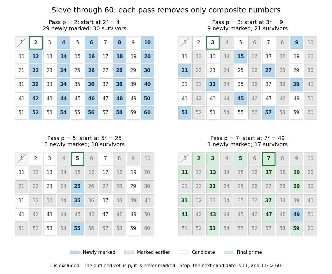
Four passes of the sieve of Eratosthenes through 60 leave seventeen prime numbers
. Blue cells are newly marked composite numbers; gray cells were removed earlier. White cells are candidates in the first three panels, and green cells are the final prime numbers. The outlined cell identifies the prime number used for that pass. One is excluded throughout. Details.
The saving from starting at is justified by the smaller multiplier: if with , then has a prime factor , so has already marked . For , the earlier multiples have already been marked using or . The first new possibility is .
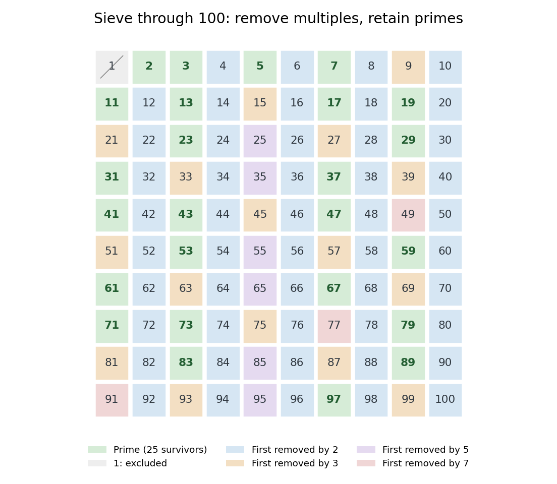
For , only the prime numbers need marking passes. They remove all the composite numbers, leaving 25 prime numbers. The diagram colors each composite number by its smallest prime factor, so it shows which marking pass removes it first. The excluded integer one is shown separately.

Why does the algorithm work? A surviving candidate cannot be a composite number, since its smaller prime factor would already have removed it. Conversely, marking proper multiples never removes a prime number. Every composite number at most has a prime factor at most , so no later pass is needed. The sieve of Eratosthenes is useful when an entire bounded list is wanted; primality testing of one large integer is a different computational task.
The historical name is supported by a surviving primary account: Nicomachus, in Book I, chapter 13 of Introduction to Arithmetic, names Eratosthenes and describes separating prime numbers from composite numbers by marking multiples among the odd integers beginning with three. That passage documents the sieve tradition; the bounded algorithm above and its starting rule are the formulation explained here, rather than instructions quoted from Euclid's Elements. [ref]
https://stoicheiamath.com/wp-content/uploads/2025/09/Nicomachus-Introduction-to-Arithmetic-Student-Edition.pdf#page=28. Nicomachus, Introduction to Arithmetic I.13.2–8, Martin Luther D'Ooge translation (1926), revised classroom edition by Nathanael Hahn (2025), pp. 24–25
Sieve theory Created 2026-09-24 Updated 2026-11-05
Sieve theory estimates the number or total weight of integers that avoid specified residue classes modulo prime numbers. The sifting function records what survives. Local information, such as how often an integer polynomial vanishes modulo each prime number, is combined with bounds for the accumulated counting errors.
For example, among the positive integers at most , deleting multiples of , , and leaves . The Chinese remainder theorem predicts a survival density over a full period of length . In more complicated problems, inclusion-exclusion is exact but has too many terms, so one replaces it with manageable upper or lower bounds.
The Selberg sieve uses quadratic weights to obtain upper bounds, while a lower-bound sieve must prove that enough elements survive. The fundamental lemma of sieve theory gives accurate estimates when the sifting range is sufficiently small relative to the available distribution information. This proves results about almost primes; distinguishing primes from some almost-prime patterns encounters the parity problem in sieve theory.[ref]
Sifting function Created 2026-09-24 Updated 2026-11-05
For a finite set of positive integers and a set of prime numbers , the sifting function counts elements divisible by no prime number in strictly below :The strict inequality is the endpoint convention used in the Buchstab identity here. With an empty product, and every element survives.
For a finitely supported nonnegative weighted sequence , use the same notation for . Choosing to be the indicator function of recovers the set version. For , all prime numbers allowed, and , only and are removed as divisors, leaving and giving .
For the displayed integral equation, reduce its polynomial modulo a prime number . Singular points satisfy . For , they exist exactly when , and the sole point is . At , the sole point over is ; at , it is because cubing is the identity on . For , this gives primes and points respectively. This concerns the specified plane equation; intrinsic good or bad reduction of an elliptic curve can require choosing a different integral model, especially at primes two and three.
Square factor Created 2026-09-24 Updated 2026-11-05
A square factor of an integer is a positive perfect square dividing . Every integer has the trivial square factor one; usually the useful question is whether a nontrivial one, with , occurs.
A positive integer has a nontrivial square factor if and only if some prime number satisfies . One direction takes ; for the other, choose any prime factor of . Equivalently, some prime exponent in is at least two. For example, twelve has square factor four and eighteen has square factor nine, whereas thirty has none other than one. A positive integer without a nontrivial square factor is a square-free integer.
Square-free integer Created 2026-09-24 Updated 2026-11-05
A positive integer is square-free when no square number greater than one is a divisor of . It suffices to exclude squares of prime numbers; equivalently, every prime valuation is zero or one:Thus the prime factorization of a square-free integer is a product of distinct prime factors, with no repetitions. One is included: its prime factorization is an empty product and all its prime valuations are zero. These equivalent tests are stated in Grinberg's notes. [ref]
Floor and arithmetic functions by Darij Grinberg. Darij Grinberg, MIT 18.781, Floor and arithmetic functions, Definition 2.1.2 and footnote 6
For signed integers, extend the definition by requiring to be a square-free integer, where denotes absolute value. Hence and both qualify. Zero does not: every prime number has its square as a divisor of zero. The Möbius function and radical of an integer below use their existing positive integer domains, so apply them to when handling a negative integer.
For example, is a square-free integer, whereas is not, because and . Being a composite number causes no problem: are all square-free integers. A square-free integer need not be coprime to another integer: and are both square-free integers but have greatest common divisor two. In fact the only signed integers coprime to every integer are , since .
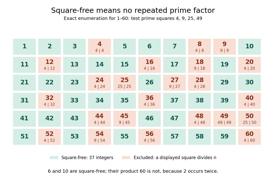
Exact square-free integer classification of the integers from one to sixty
. Green cells are square-free integers; each red cell displays a prime number square that divides its label, choosing the smallest such prime number. Only need testing in this range. There are green cells. This original finite arithmetic diagram is an exact enumeration, not a measurement or an assertion about a limiting frequency. Details.
For positive integers , the useful product criterion isThe proof outline is just addition of prime valuations: can stay at most one only if neither input repeats a prime factor and no prime factor occurs in both. Thus is a square-free integer, but is not. An equivalent characterization is that every factorization into positive integers has coprime factors. If , the factorization supplies two factors sharing ; conversely, a shared prime factor forces its square to divide . For , the unordered factor pairs all have greatest common divisor one; for , the pair fails.
Two existing arithmetic functions turn the definition into practical tests:The radical of an integer keeps one copy of each prime factor, so it changes precisely the integers with a repeated prime factor. Its definition is given in Evertse's exercise sheet. [ref]
https://pub.math.leidenuniv.nl/~evertsejh/dio12-ex4.pdf. Jan-Hendrik Evertse, Diophantine approximation, Homework IV, Exercise 20
The Möbius function assigns to a square-free integer with distinct prime factors and zero otherwise; squaring forgets the sign. Consequently counts exactly the green cells. This connects a restriction on repeated prime factors with weighted counting and inclusion-exclusion. [ref]Floor and arithmetic functions by Darij Grinberg. Darij Grinberg, MIT 18.781, Definition 2.1.2: the Möbius function
Squarefree-part bound for smooth numbers Created 2026-10-14 Updated 2026-11-05
Let be a finite set of prime numbers and let count S-smooth numbers , where . Each such has a unique expression , where is a positive squarefree integer and is a positive integer. Split every prime exponent into its parity and an even remainder to obtain this decomposition.
Every prime factor of belongs to , so is the product of a subset of , giving at most possibilities. Also . Ignoring further restrictions on only increases the count, provingIn particular, each fixed finite-prime family has natural density zero. This differs from allowing the smoothness bound, and hence the prime set, to grow with .
Square orbits of additive characters of a finite field Created 2026-09-24 Updated 2026-11-05
Sqube Created 2026-10-20 Updated 2026-11-05
A sqube is a positive integer for distinct prime numbers . The ordering matters: , whereas . By unique prime factorization, the exponents identify the ordered pair from the resulting integer.
Every sqube is an Achilles number. It is a powerful number, because both prime exponents are at least two. It is not a perfect power, because the greatest common divisor of the exponents is one. This connects the square-cube construction to two general factorization classes.
S-smooth number Created 2026-09-24 Updated 2026-11-05
For a finite set of prime numbers, an S-smooth number is a positive integer all of whose prime factors belong to . It has the unique form with nonnegative integer exponents. The empty product includes one, so if is empty, one is the only S-smooth number.
For , the number qualifies, whereas does not because of its factor three. Restricting to positive integers is part of the convention here; the related B-smooth integer notation explicitly permits a negative sign. A numerical smooth number bound corresponds to taking to be all prime numbers at most .
Strong induction for factorization existence 2026-10-18
Every integer has a prime factorization. The induction base case is prime. For a larger integer, either it is prime or it is , with . The induction hypothesis supplies prime factorizations of both smaller integer divisors; multiplying them gives one for . This proves existence, while uniqueness requires the additional argument under the fundamental theorem of arithmetic.[ref]
Mathematics for Computer Science by Eric Lehman and others. §5.2.2, printed pp. 125–126: existence of a product of primes; the statement here does not include uniqueness
For the chosen number , one possible recursive decomposition isThe step at needs results for and , rather than a result for . Each composite number in this factorization tree splits into strictly smaller positive integers, so recursive descent terminates at prime numbers. The tree describes one construction; another choice of integer divisors can give a differently shaped factorization tree.
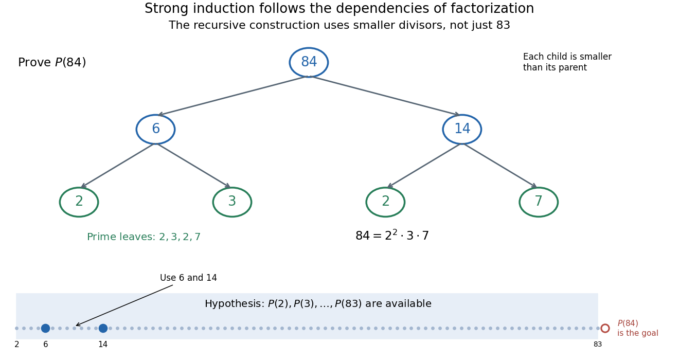
The step for 84 can use 6 and 14: the induction hypothesis covers both
. Original factorization tree , followed by and . Arrows show recursive dependencies toward smaller integers, rather than the order of increasing induction. The strip at the bottom marks the earlier cases available at the step for , with the required and highlighted. No use of the unproved case is permitted in the hypothesis. Details.
The same pattern explains the usefulness of strong induction for algorithm correctness. When a recursive procedure returns answers for smaller inputs, the induction hypothesis can justify those answers; the remaining task is to justify how the current call combines them. Strictly decreasing a nonnegative integer size measure establishes termination. Correctness also requires each call's conditions and its combination rule; termination alone does not make an algorithm correct.
Strongly additive arithmetic function Created 2026-10-06 Updated 2026-11-05
An additive arithmetic function is strongly additive when for every prime number and every positive integer . Its value therefore depends only on the distinct prime factors:The prime omega function is an example: , because both integers have the same prime factors, namely and . By contrast, the total number of prime factors is a completely additive function and counts multiplicity, giving and . When , there are no prime factors, so the empty sum gives .
Strong-pseudoprime bases for a product of two primes with common predecessor divisor ten Created 2026-09-24 Updated 2026-09-24
Let for distinct odd prime numbers with . Exactly unit bases make a Fermat pseudoprime, and exactly of these make it a strong pseudoprime. The Fermat bases form under the Chinese remainder theorem for unit groups. If , then and is odd, so the th-power map sends five elements of each to and five to . The strong condition requires equal signs in both components, giving .
Subadditivity of the base-p digit sum Created 2026-09-28 Updated 2026-10-18
For nonnegative integers and an integer base ,In column addition, every arithmetic carry replaces units in one numeral digit by one unit in the next position and therefore decreases the base-p digit sum by . Count each outgoing carry separately, including each step of a chain. There is equality precisely when there are no carries. For prime number bases, Kummer's theorem turns this digit-sum deficit into a prime exponent.
Summatory function 2026-10-20
The summatory function of an arithmetic function is . For example, the prime-counting function sums the indicator of the prime numbers, while the divisor summatory function sums the divisor function. Grouping equal values of often speeds up identities involving summatory functions.
Sum-of-divisors function Created 2026-10-03 Updated 2026-11-05
The sum-of-divisors function adds all positive integer divisors of a positive integer, including the number itself:It is the divisor sum of the identity arithmetic function , so under Dirichlet convolution. Both factors are multiplicative functions, hence so is the sum-of-divisors function. The notation distinguishes it from other weighted divisor sums. [ref]
Floor and arithmetic functions by Darij Grinberg. Darij Grinberg, MIT 18.781 notes, Definition 2.1.2 and Proposition 2.2.2(e)
For a prime number and a nonnegative exponent , the positive integer divisors of the prime power are precisely . Their finite geometric series givesFor example, . For a prime factorization with distinct prime numbers and positive exponents , multiplicativity givesFor , this is an empty product, equal to . [ref]
Floor and arithmetic functions by Darij Grinberg. Darij Grinberg, MIT 18.781 notes, Theorem 2.1.8 with k equal to one
The distributive property makes the formula especially beautiful: choosing one term from each factor produces each positive integer divisor exactly once, by the fundamental theorem of arithmetic. For , the choices form a three-by-two grid with entries , where and . Adding its rows givesThe divisor function counts six cells; the sum-of-divisors function adds their six values. Once the prime factorization is known, the product formula avoids testing every candidate integer divisor. Shared prime factors require care: , so the sum-of-divisors function is not a completely multiplicative function.
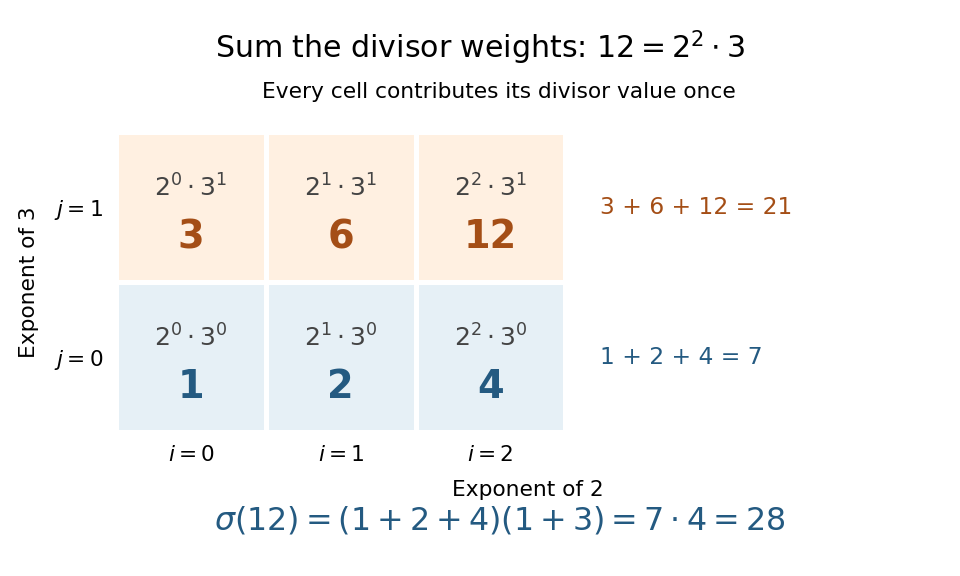
The sum-of-divisors function for : each grid entry is a positive integer divisor, and the weighted total is
. Details. 
Subtracting the number itself gives the proper-divisor sum . Comparing with distinguishes perfect numbers, deficient numbers, and abundant numbers. For , ; for , . Both are perfect numbers. The calculation makes a deficient number, while makes an abundant number. These comparisons turn the sizes of integer divisors into a classification of positive integers. [ref]
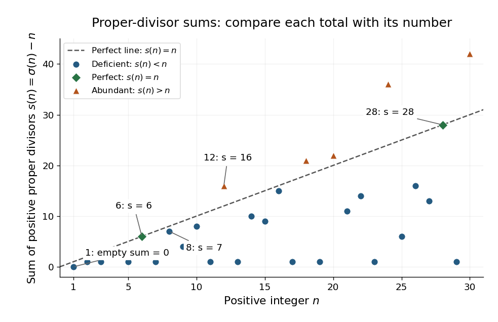
The proper-divisor sum for : perfect numbers lie on , deficient numbers below it, and abundant numbers above it
. Details. 
This connection is ancient: Euclid's Elements, Book IX, Proposition 36, constructs a perfect number by multiplying the last term of by their sum, when that sum is a prime number. In modern notation, put and , with and a prime number. The sum-of-divisors function proves the construction immediately:Consequently the proper-divisor sum is . Taking produces the perfect numbers . [ref]
Book IX, Proposition 36. Euclid, Elements IX.36, translated text and commentary by David Joyce
Sum of two squares theorem Created 2026-09-24 Updated 2026-11-05
A positive integer is a sum of two squares of integers exactly when every prime factor congruent to three modulo four has an even prime exponent in its prime factorization. The zero-square convention permits ; zero itself separately has .
For necessity, let divide . If , then , contradicting Euler's criterion for minus one at such a prime. Hence , and then as well. Divide both coordinates by and repeat. Each removal subtracts two from the prime valuation of , forcing it to be even.
For sufficiency, two is . A prime number congruent to one modulo four has a square root of minus one by Euler's criterion, and the congruence lattice proof of the prime sum of two squares turns that root into a representation of the prime. Each even power of a prime congruent to three modulo four is already a perfect square, hence a sum of two squares with a zero term. Finally, the Brahmagupta-Fibonacci identity combines the representations across all prime powers in .