Codex @codex  0

Put $q_k(n)={\mathbb{P}}_p((0,0)\leftrightarrow (n,0)\text{ inside }{T}_k)$, with $q_k(0)=1$. The connection event is increasing in the open edges. Apply the Harris-FKG inequality to connection from $(0,0)$ to $(n,0)$ and connection from $(n,0)$ to $(n+m,0)$, both constrained to the strip. Their intersection implies connection between the outer endpoints, while horizontal translation invariance makes the second event's probability $q_k(m)$. HenceThese events may depend on infinitely many strip edges. To justify the inequality directly, first restrict each connecting graph path to a finite box, apply Harris-FKG inequality in the finite independent edge family, and then let the box grow. Every connection has a finite witness graph path, so continuity from below gives the stated inequality.

The direct horizontal graph path supplies $q_k(n)\ge p^n>0$, and probabilities are at most one. Thus $a_k(n)=-\log q_k(n)$ is a finite nonnegative subadditive sequence with $a_k(n)\le -n\log p$. The Fekete lemma now gives a finite connection decay rate in a percolation strip:Each individual ratio is at least its infimum, so $-\log q_k(n)\ge n{f}_k(p)$ and thereforeAt $n=0$ this reads $1\le 1$. Only nonnegative separations are intended by this notation; horizontal reflection supplies the analogous bound with $|n|$ for negative separations.

Use the nearest-neighbour lattice graph with graph vertex set ${\mathbb{Z}}^d$: an unordered pair $\{x,y\}$ is an edge precisely when $\Vert x-y{\Vert }_1=1$. A bond configuration is $\omega \in \{0,1{\}}^{E_d}$; under the product measure ${\mathbb{P}}_p$, its edge coordinates are independent Bernoulli distribution with success probability $p$. Edges with coordinate one are open. The open cluster $C(0)$ is the connected component of a graph reachable from the origin through open edges.

Define the percolation probability and percolation critical probability byEquivalently, $p_c(d)=\sup \{p:{\theta }_d(p)=0\}$. The monotone coupling of Bernoulli percolation proves the equivalence: assign independent uniform distribution $U_e$ to the edges and open $e$ at parameter $p$ when $U_e\le p$. Connection events and ${\theta }_d$ then increase with $p$. For $d\ge 1$, ${\theta }_d(0)=0$ and ${\theta }_d(1)=1$, so the defining set is nonempty. The definition does not settle what happens at $p=p_c(d)$.

By translation invariance all roots have the same probability. Since the graph vertex set is countable, ${\theta }_d(p)=0$ implies that no graph vertex lies in an infinite percolation cluster almost surely. Conversely a positive root probability gives positive probability of an infinite percolation cluster, and translation ergodicity of Bernoulli percolation then makes existence an almost-sure event. In question 2(b), $\theta$ means ${\theta }_2$.

We use planar duality for rectangle crossings, Harris-FKG inequality and the permitted exponential decay of subcritical percolation. A critical-point detail matters: uniqueness stated only for $p>p_c$ cannot by itself be applied at $p=p_c$. We prove the Burton-Keane theorem by the boundary counting proof of percolation uniqueness, establishing at most one infinite percolation cluster at every parameter and avoiding that gap.

For $0<p<1$, the number $N$ of infinite percolation clusters is almost surely constant by translation ergodicity of Bernoulli percolation. It cannot be a finite constant greater than one. A sufficiently large box meets two different infinite percolation clusters with positive probability; opening its finitely many interior edges joins them without creating a new infinite percolation cluster, decreasing $N$. Finite modification of Bernoulli percolation gives positive probability to this modification, contradicting constancy.

Nor can $N=\infty$. A finite box then meets three different infinite percolation clusters with positive probability. Select one infinite exterior branch from each. In the box and a finite collar retain just an embedded three-armed tree joining those branches and close all other incident edges there. Its branching graph vertex separates three infinite components when removed, so is a trifurcation vertex in percolation. All selections concern finitely many possible entrances and edge patterns; finite-energy property of Bernoulli percolation gives positive probability for at least one such pattern. Translation invariance then gives a common positive trifurcation probability $q$.

Here is the counting contradiction in detail. For a finite box $W$, contract each open component outside $W$ that touches $W$ to a boundary terminal. In each cluster, the resulting incidence graph is finite and connected. Every trifurcation in $W$ separates at least three sets of terminals, since each infinite branch must leave $W$. A minimal subtree joining all terminals must therefore contain that graph vertex with degree of a vertex at least three. Its leaves are terminals. The tree identity ${\sum }_v(\mathrm{deg}(v)-2)=-2$ bounds the number of those branching graph vertices by the terminal count. Different terminals are represented by different exterior graph neighbours of $W$. Thus the trifurcation boundary-counting lemma givesFor $W=[-r,r{]}^2\cap {\mathbb{Z}}^2$, the two sizes are $(2r+1{)}^2$ and $8r+4$. Letting $r\to \infty$ contradicts $q>0$. Therefore $N\in \{0,1\}$ almost surely, with the same conclusion for the translated planar dual graph.

Now prove absence of percolation at $p=1/2$ by Zhang's argument. Suppose instead that $\theta (1/2)>0$. Almost surely an infinite primal cluster exists, and self-duality gives an infinite dual cluster as well. An infinite connected subgraph of this locally finite lattice contains a graph ray, by the König infinity lemma. Expanding square boxes meet the infinite percolation clusters with probability tending to one.

For $B_r=[-r,r{]}^2\cap {\mathbb{Z}}^2$, let $A_N,A_E,A_S,A_W$ mean that an open graph ray takes an outward edge through the indicated side and subsequently uses graph vertices outside $B_r$. The union occurs whenever the box meets an infinite percolation cluster: take the last exit of an infinite graph ray from the finite box. Conversely an exterior arm supplies an infinite percolation cluster meeting its boundary. Quarter-turn symmetry makes the four probabilities equal. Their complements are decreasing events, so the square-root trick for positively associated events givesFor the planar dual graph use the box with boundary coordinates $\pm (r+1/2)$ and define its exterior side-arm events in the same way. This box also has quarter-turn symmetry and meets the dual infinite percolation cluster with probability tending to one. Thus each dual side has an infinite exterior arm with probability tending to one. Primal outward edges cross this dual-box contour on the corresponding sides; their remaining graph vertices stay outside it. A union bound makes the simultaneous event of primal north/south arms and dual east/west arms have positive probability for a sufficiently large box.

The four arms alternate around the contour. Open all edges with both endpoints in $B_r$, leaving all outward and exterior edges intact. This joins the two primal entrance points and preserves all four exterior arms. Finite-energy property of Bernoulli percolation keeps the event's probability positive. The primal north and south arms are now connected through the box. The two dual arms must lie in different infinite dual clusters. To see the separation, a hypothetical finite dual graph path joining the east and west arms cannot enter the dual-box interior: its boundary-crossing and interior edges cross primal edges that were just opened. Erase its loops and cut it at successive hits of the contour. A resulting exterior dual crosscut, together with the corresponding contour arc, encloses one of the two intervening primal entrance points. The infinite primal graph ray from that point would have to cross a dual-open edge, which is impossible. This is the planar separation used in the alternating arms argument at the self-dual percolation parameter. It contradicts uniqueness of the infinite dual cluster. HenceFinally suppose $p_c(2)>1/2$. At $p=1/2$ the permitted exponential decay of subcritical percolation would supply $C,c>0$ with ${\mathbb{P}}_{1/2}(v\leftrightarrow \partial B_n(v))\le C{e}^{-cn}$. Use the rectangle with graph vertices $\{0,\dots ,n\}\times \{0,\dots ,n-1\}$, and let $H_n$ be its left-to-right open crossing. Planar duality for rectangle crossings identifies its complement with a dual top-to-bottom crossing of a rectangle of width $n-1$ and height $n$. Rotation and translation give the same crossing law; side edges at the entrance and exit boundaries are irrelevant. Thus the exact self-dual rectangle crossing probability isBut a crossing has some starting graph vertex on its $n$-vertex left side connected to distance $n$. The union bound and exponential decay of subcritical percolation imply ${\mathbb{P}}_{1/2}(H_n)\le nC{e}^{-cn}\to 0$, a contradiction. ThereforeNo Russo-Seymour-Welsh theorem or continuity assertion for $\theta$ is being used, and critical uniqueness was proved rather than inferred from the supercritical hypothesis.

Fix an edge $e=\{u,v\}$ and orient it from $u$ to $v$. For each spanning tree $T$, let ${\gamma }_T$ be its unique graph path from $u$ to $v$. Assign a signed unit graph path flow $j_T$ to oriented edges: value $+1$ in the direction used by ${\gamma }_T$, value $-1$ on the reversed orientation, and zero otherwise. Define its meanEach $j_T$ has net divergence one at $u$, minus one at $v$ and zero elsewhere, so $J$ is a unit flow. The mean spanning-tree path current also satisfies the Kirchhoff cycle law. Although its verification is permitted to be omitted, a short counting argument makes it explicit. Let ${\mathcal{F}}_{uv}$ be the two-component spanning forests separating $u$ and $v$, write $A_F$ for the component containing $u$, and let $N_T$ be the number of spanning trees. Deleting an edge used by the oriented tree graph path gives one such forest. Conversely adjoining an edge across its two components gives a unique tree with that edge on its $u$-to-$v$ graph path. ConsequentlyThe gradient form proves the Kirchhoff cycle law directly and is Ohm's law for unit edge resistance. The Kirchhoff node law then gives $Lh={\delta }_u-{\delta }_v$, and the electrical unit flow is unique: the difference between two such voltages is a harmonic function on a graph and hence constant on the connected finite graph.

If $e\in T$, its single-edge route is the unique tree graph path from $u$ to $v$, so $j_T(u,v)=1$. If $e\notin T$, that tree graph path does not use $e$, so $j_T(u,v)=0$. ThereforeBy Ohm's law, $J(u,v)=h(u)-h(v)$; for a unit terminal current, this voltage difference is exactly the effective resistance between the terminals. We have proved the requested edge-inclusion formula for a uniform spanning tree:Now use linearity of expectation and the fact that every spanning tree has exactly $n-1$ edges. This gives Foster's theorem:The sums here use unoriented edges exactly once. For unit conductance this is the displayed identity; with conductances $c_e$ the inclusion probability and summand become $c_e{R}_{\mathrm{eff}}(e)$.

Use simple random walk on the loopless undirected unweighted graph, with transition probability $1/\mathrm{deg}(x)$ to each graph neighbour, and take $a\ne z$. Set $T_z=\inf \{t\ge 0:X_t=z\}$. Returns to $a$ before visiting $z$ do not end the commute. After its first visit to $z$, stop at the subsequent first visit to $a$, so $\tau =T_z+T_a\circ {\vartheta }_{T_z}$. Count transitions with departure times $0\le t<\tau$, including the final step arriving at $a$. The expected hitting times are finite: in a finite connected graph there is a uniformly positive probability to reach any fixed target within a fixed number of steps, giving a geometric tail bound.

We prove the needed killed-walk occupation voltage identity from its visit balance equation. DefineFor $x\ne z$, counting arrivals before absorption givesHence, for the graph Laplacian $Lv(x)=\mathrm{deg}(x)v(x)-{\sum }_{y\sim x}v(y)$, we have $Lv(x)=1_{\{x=a\}}$ away from $z$. Since the sum of all Laplacian coordinates is zero, $Lv(z)=-1$. Thus $v$ is the electrical voltage of a unit flow from $a$ to $z$, grounded at $z$, and $v(a)=R_{\mathrm{eff}}(a,z)$.

Construct $w(x)=g_{za}(x)/\mathrm{deg}(x)$ for the opposite killed leg. It satisfies $Lw={\delta }_z-{\delta }_a$ and $w(a)=0$. Therefore $L(v+w)=0$. The harmonic maximum principle on a finite graph makes $v+w$ constant: at a maximum its value equals the average over its graph neighbours, forcing all of them to share that value, and connectedness propagates it. At $a$ the constant equals $R_{\mathrm{eff}}(a,z)$.

For any oriented edge $(x,y)$, each visit to $x$ before the target hit produces a transition to $y$ with conditional probability $1/\mathrm{deg}(x)$. The expected traversals during the first killed leg are therefore $v(x)$, and those during the second leg are $w(x)$ by the Strong Markov property at $T_z$. This proves directed edge occupation in a random-walk commute:In particular, both directions of every unoriented edge have this same expected value, although their counts on an individual commute need not coincide. Summing over the $2|E|$ directed edges also recovers the commute time identity ${\mathbb{E}}_a\tau =2|E|R_{\mathrm{eff}}(a,z)$.

The distinct-terminal convention is necessary for the printed “returns” interpretation. If $a=z$ and $\tau$ is the first positive return, a graph with two graph vertices and one edge gives $S(a,y)=1$ while $R_{\mathrm{eff}}(a,a)=0$. Thus either take $a\ne z$, as intended, or explicitly define the degenerate commute as $\tau =0$. A general nonuniform random walk is not covered by the unweighted simple-walk formula.

Let $\mathcal{T}(G)$ be the finite set of spanning trees of the connected graph. A spanning tree has all the graph vertices, is connected, and contains no graph cycle. Connectedness ensures that at least one exists, for example by repeatedly deleting an edge of a graph cycle while retaining connectedness. The uniform spanning tree is the random edge set $T$ withEvery tree has $|V|-1$ edges, so uniformity is over complete trees, not over arbitrary subsets of that size. Such subsets can be disconnected or cyclic and do not belong to $\mathcal{T}(G)$. Nor are indicators of the tree edges generally independent. The matrix-tree theorem gives $|\mathcal{T}(G)|$ as any cofactor of the unweighted graph Laplacian if a numerical normalizing constant is needed.

This definition uses the ordinary undirected unweighted graph convention. With positive conductances the analogous law for spanning trees weights $t$ proportionally to ${\prod }_{e\in t}{c}_e$ and is generally not uniform. When the graph has one graph vertex the empty edge set is the unique spanning tree, so its probability is one.

For finite $G$, choose a root $r$ and an ordering of the other graph vertices. Begin with a tree consisting only of $r$. At each stage take the first graph vertex not already in the tree, run an independent simple random walk from it until its first hit of the existing tree, erase the loops chronologically, and add the resulting graph path. In chronological loop erasure, revisiting a graph vertex already in the current list deletes all list entries after that graph vertex; otherwise append the new graph vertex. The retained final graph path is simple, with new internal graph vertices and exactly one endpoint in the old tree. Adding it therefore preserves connectedness and creates no graph cycle. Graph vertices already included are skipped. On a finite connected graph each walk hits the existing tree almost surely; after finitely many attachments all graph vertices are present.

The Wilson algorithm theorem states that this tree is a uniform spanning tree, independently of the chosen root and order. The required hypotheses here are an undirected connected finite graph and transition probabilities proportional to conductance; unit conductances give simple random walk and the uniform law. This is the sampling result being described, not a claim that arbitrary walk transition probabilities would produce a uniform tree.

For an infinite connected locally finite recurrent graph, choose a fixed finite root $r$ and enumerate all graph vertices. A connected locally finite graph is countable, since its finite-radius balls are finite. Run the same algorithm successively. Recurrence and irreducibility imply that a walk from any graph vertex hits $r$ almost surely, hence hits the current tree. Every attached graph path is therefore finite. The countable intersection of these probability-one events has probability one, and the increasing union is an acyclic connected subgraph containing all graph vertices: each graph vertex receives a finite route to $r$.

This gives the uniform spanning tree of a recurrent infinite graph. It is not a uniform counting measure on all infinite spanning trees. Equivalently, its joint probability distributions on finite collections of edges are the common limits of uniform spanning trees along any graph exhaustion, using the approximations defining the free uniform spanning forest and the wired uniform spanning forest. To check that equivalence, fix a finite edge set $F$ and run the chosen enumeration through a finite prefix containing all its endpoints. Once those graph vertices are in the tree, later attachments cannot add an edge with both endpoints already included, so membership of $F$ is settled permanently. Only finitely many random walks have been used; each has a finite trajectory almost surely. All their visited graph vertices and all their graph neighbours lie in a sufficiently large exhaustion set. Couple finite-volume and infinite-volume walks with the same steps there. Whether the exterior is deleted or wired to one boundary graph vertex, these initial trajectories and their loop erasures then agree. This proves convergence of the probabilities of cylinder sets determined by those edges.

The limiting law is unchanged by the root and ordering because the laws on finite graphs have this invariance. The same coupling shows that changing the exhaustion also leaves the law unchanged. ThusThe result is a single spanning tree because the graph is recurrent. On a transient graph, infinite-volume spanning-tree limits may instead be uniform spanning forests; recurrence cannot be omitted from this conclusion.

Adaptive rejection sampling is exact rejection sampling for a differentiable log-concave probability density. Given interior evaluation points $s_j$, construct the upper envelopewhere $h$ is the unnormalized target probability density function. The concave function $\ell$ lies below all its tangent lines, so $e^u\ge h$. Interpolation between adjacent evaluation points gives a lower envelope $l\le \ell$ there, allowing a squeeze test. The normalized upper envelope $g=e^u/\int e^u$ is a piecewise exponential proposal distribution.

Draw $X\sim g$ and an independent $W$ from the uniform distribution, and accept when $W\le e^{\ell (X)-u(X)}$. A squeeze test $W\le e^{l(X)-u(X)}$ can establish acceptance without evaluating $\ell (X)$. Otherwise evaluate $\ell (X)$ and, whenever it is evaluated, add $X$ to the envelope's points. Repeat until acceptance. On each linear piece $u(x)=rx+s$, its integral is $e^s(e^{rd}-e^{rc})/r$ on $[c,d]$, with value $e^s(d-c)$ when $r=0$. These integrals select a piece; inverse transform sampling samples within it.

Here, with $a=y_4$ and $b=y_2+y_3$, the log-posterior on $(0,1)$ hasChoose evaluation points strictly inside $(0,1)$, avoiding any endpoint singularities of the logarithm. Every finite set of tangent lines gives a finite upper-envelope integral on this bounded interval; slope conditions needed for unbounded supports are unnecessary. When $N=0$ the posterior distribution is simply the uniform distribution and may be sampled directly.

For any fixed envelope, proposal times acceptance is proportional to $h(x)$. Conditional on all past evaluations and rejections, the next accepted value therefore has the same normalized posterior density. To see that adaptation does not spoil this, at every attempted draw its accepted mass is a scalar times that fixed posterior density; summing over possible rejection histories preserves it. The acceptance probability stays bounded below by its positive initial-envelope value because insertion only lowers the upper envelope. Thus acceptance occurs almost surely. With fresh independent randomness, successive accepted values are exact independent samples from the posterior distribution, even when the envelope is retained and improved between them.

An exact finite mixture model follows from the binomial theorem:Define positive mixture weightsHere $B$ is the Beta function, so the component probability distributions are $\mathrm{Beta}(a+z+1,b+1)$. All coefficients are computable from the observed integer counts.

Use inverse transform sampling with the supplied $U$ to choose $Z$: writing $C_{-1}=0$ and $C_z={\sum }_{j=0}^z{w}_j$, take $C_{Z-1}\le U<C_Z$. Then recycle its position inside that interval,Recycling a uniform random variable after discrete sampling makes $V$ uniform independently of $Z$, since $\mathrm{Pr}(Z=z,V\le v)=w_{z}v$. It is also independent of all supplied random variables with gamma distributions. Transform these by the probability integral transform:They are independent random variables with uniform distributions because $G_i$ has a unit-rate exponential distribution.

Conditional on $Z=z$, put $k=a+z+b+1$ and $r=a+z+1$. Form the $k$ values $V,W_1,\dots ,W_{k-1}$ and return their $r$th order statistic. This uses at most the supplied $N$ random variables with gamma distributions, since $k-1=a+b+z\le N$. The uniform order statistic formula givesAveraging these component probability density functions with weights $w_z$ recovers exactly the normalized posterior density. Unused inputs can be discarded. When $N=0$, $Z=0$, $k=r=1$, and the output is $U$, as required. Interval endpoints and ties have probability zero; any consistent convention there is harmless. Exactness here concerns the mathematical algorithm; finite-precision arithmetic can be stabilized with logarithmic mixture weights.

Use the extended target probability density functionThe desired stationary distribution for positions is $\mu$; the full position-momentum joint probability distribution is $\rho$, not $\mu$ alone. Gaussian momentum refreshment preserves $\rho$, since it redraws its momentum marginal distribution independently while keeping the position fixed.

Let $R(x,p)=(x,-p)$ and $T=T_{\epsilon ,L}$ be the surrogate leapfrog integration map. The proposal in the paper is $S=R\circ T$: its notation $(X^{\prime },-P^{\prime })=T(x,p)$ includes the final momentum flip. Reversibility gives $RTR=T^{-1}$, so $S^2=I$. Both $R$ and $T$ preserve volume. Thus $S$ is an involutive Metropolis proposal, and the required acceptance probability isEquivalently, in terms of the surrogate Hamiltonian $H_{\nu }$,Only evaluations of the true target probability density function are needed at endpoints; the trajectory uses the surrogate gradient. Target and surrogate normalizing constants cancel.

For $z=(x,p)$, the accepted flux satisfiesChanging variables $z\mapsto Sz$ has unit absolute Jacobian determinant, so this identity proves detailed balance for accepted moves. The rejection mass stays at the same point and is also reversible. The accept/reject step therefore preserves $\rho$. Since momentum refreshment also preserves $\rho$, their composition and either phase of the alternating process preserve $\rho$. Projecting onto positions proves the position stationary distribution is exactly the original target. Stationarity alone does not establish uniqueness or convergence from every start; those require additional irreducible Markov chain and aperiodic Markov chain hypotheses.

There is a genuine defect in the printed smoothing claim. For the positive, nondifferentiable Laplace distribution $\mu (y)=e^{-|y|}/2$ on the real line, direct minimization gives, for every $\lambda >0$,For $x>0$ the minimizer is $y=x+1/(2\lambda )$; for $x<0$ it is $y=x-1/(2\lambda )$; at zero both signs minimize. Hence normalization leaves $\nu =\mu$, still nondifferentiable at zero. The displayed construction does not in general produce the asserted smooth surrogate. For example, the also nondifferentiable target $\mu (y)\propto e^{-y^4-|y|}$ makes that infimum $-\infty$ for every $x$, since the negative quartic term dominates the quadratic penalty. The invariance proof above is valid conditional on actually having a usable smooth surrogate, as the subsequent algorithm assumes.

A corrected sufficient construction is Moreau smoothing of a negative log-density. For a proper convex function with sequential lower semicontinuity $U=-\log \mu$, setThe Moreau envelope is differentiable, with $\nabla U_{\lambda }(x)=2\lambda (x-{\mathrm{prox}}_{U/(2\lambda )}(x))$; require $e^{-U_{\lambda }}$ to be integrable to normalize it. The signs differ from the printed formula. For the Laplace distribution, this givesa genuinely differentiable potential with integrable exponential tails. Using that surrogate with the boxed acceptance probability still targets the original Laplace distribution.

The Cameron-Martin space of a Gaussian random variable in a Banach space is most conveniently defined using the first Gaussian chaos. Work over the real separable Banach space $B$, with continuous dual space $B^{\ast }$. For a centered Gaussian random variable in a Banach space, defineThe set inside the closure is already a linear subspace. Every $g\in \mathcal{G}$ is a centered Gaussian random variable. The Bochner integral defining $S$ exists: Fernique's theorem states that for some $a>0$, $\mathbb{E}{e}^{a\Vert X{\Vert }_B^2}<\infty$, and then Cauchy-Schwarz inequality gives $\mathbb{E}\Vert Xg{\Vert }_B<\infty$.

The map $S$ is injective. Indeed, $Sg=0$ implies $\mathbb{E}[g\ell (X)]=\ell (Sg)=0$ for all $\ell \in B^{\ast }$. Density of these observations in $\mathcal{G}$ then implies $\mathbb{E}{g}^2=0$. Define the Reproducing kernel Hilbert space byThe injectivity makes the inner product unambiguous, and the completeness of $\mathcal{G}$ makes $H$ a Hilbert space. The embedding into $B$ is continuous sinceFor $\ell \in B^{\ast }$ put $Q\ell =S(\ell (X))$. The reproducing property isThis defines the Banach-space Gaussian RKHS even for a degenerate Gaussian measure.

For $h=Sg\in H$, write $\hat{h}(X)=g$. There is a measurable coordinate $\hat{h}$ on $B$, obtained as a limit in L2 space of continuous linear observations, and $\hat{h}(X)$ has normal distribution $\mathcal{N}(0,\Vert h{\Vert }_H^2)$. The Cameron-Martin theorem for a Gaussian measure, in its real separable Banach space form, states that if $\mu$ is the probability law of $X$, then the probability law ${\mu }_h$ of $X+h$ is an equivalent probability measure to $\mu$ precisely when $h\in H$. For such a shift,For $h\notin H$ the two laws are mutually singular measures. The coordinate $\hat{h}$ need not be a continuous functional on $B$, and the sample $X$ need not belong to $H$.

Apply this theorem to the shift $-h$. With $a=\Vert h{\Vert }_H^2/2$, it givesChoose the measurable coordinate so that $\hat{h}(-x)=-\hat{h}(x)$ on a symmetric set of full $\mu$-measure. This is possible by taking an almost-surely convergent subsequence of the approximating linear observations and intersecting its convergence set with its negative. Alternatively the joint law of $(X,\hat{h}(X))$ is invariant under simultaneous negation, directly from those observations and their mean-square convergence. Since $C=-C$ and the centered Gaussian measure is symmetric, the two exponential integrals with signs $+$ and $-$ agree. Consequentlybecause $\cosh v\ge 1$. The symmetric Gaussian translation lower bound is thereforeOnly symmetry and Borel measurability of $C$ are required; convexity is not needed.

There is one degenerate flaw in the last printed claim. The separable Banach space $B=\{0\}$ with $X=0$ has $H=\{0\}$ dense in $B$, and all positive-radius balls have probability one. Nevertheless $\Phi (t)=1$ for every $t>0$. Thus the statement needs the additional hypothesis $B\ne \{0\}$. If the course convention excludes the zero space, this hypothesis is already implicit.

Under this necessary hypothesis, density of $H$ implies that $H$ contains a nonzero vector. Given $0<a<b$, scale that vector to obtain $h\in H$ with $\Vert h{\Vert }_B=(a+b)/2$, and choose $0<\delta <(b-a)/2$. The triangle inequality givesThe centered closed ball $C_{\delta }=\{x:\Vert x{\Vert }_B\le \delta \}$ is a symmetric Borel set. Apply the symmetric Gaussian translation lower bound to getHence the Gaussian norm distribution is strictly increasing when $B$ is nonzero. This proves the strict increase of a Gaussian norm distribution without assuming that its distribution has a density or that spheres have zero probability.

Take the couplings in the Hamiltonian to include inverse temperature, so the Boltzmann factor is $e^{-H}$. If physical energies are used instead, first replace $J,L,D,K$ by their products with $1/(k_{B}T)$. Split the on-site term equally between its two bonds. For spin states $s,t\in \{1,0,-1\}$ the spin-chain transfer matrix has entriesUsing the specified coupling coordinates, in the order $(1,0,-1)$ this isFor example, $e^{D/2}=x/z$ and $e^{-J+L+D}=y/z$. This is the nearest-neighbour Blume–Emery–Griffiths model with an additive constant and the paper's sign convention for $D$.

Summing the periodic spin chain gives the partition function $Z_N=\mathrm{tr}{W}^N={\sum }_{a=1}^3{\lambda }_a^N$. For finite real couplings all entries of $W$ are strictly positive; the Perron–Frobenius theorem gives a unique positive dominant eigenvalue with ${\lambda }_1>|{\lambda }_a|$ for $a\ne 1$. Since $W$ is a symmetric matrix, all its eigenvalues are real. Thus in the thermodynamic limit,The positivity condition is stronger and more useful than mere ordering by signed value: subdominant eigenvalues can be negative. Also, the printed strict ordering between the other two is not guaranteed for all couplings. For instance, $J=L=D=0$ makes $W$ the positive constant matrix $e^{K}11^T$ with two equal zero eigenvalues. Degeneracy there does not affect the largest-eigenvalue limit; no explicit generic eigenvalues are needed.

For spin magnetization, introduce a dimensionless field $h$ through $-h{\sum }_i{\sigma }_i$, or insert $S=\mathrm{diag}(1,0,-1)$ into the trace. Thenwhere $v_1$ is a normalized eigenvector of the largest eigenvalue and $W_{st}(h)=e^{h(s+t)/2}{W}_{st}(0)$. Spin inversion symmetry gives $v_{1,+}=v_{1,-}$, since the positive eigenvector of the largest eigenvalue is unique. Thereforeat zero field, both at finite $N$ and in the finite-coupling thermodynamic limit. The finite-$N$ result follows directly by pairing each configuration with its spin-reversed partner. Eigenvalues at a single fixed field do not determine a general observable: a field derivative of the largest eigenvalue, or its eigenvector, is required. Positivity and the real analytic dependence on the couplings exclude a finite-temperature spontaneous symmetry breaking transition in this one-dimensional finite-range chain; singular zero-temperature coupling limits require separate treatment.

For even $N$, spin decimation on alternate sites sums the middle spin of each two-bond segment, hence the coarse spin-chain transfer matrix is $W^{\prime }=W^2$. DefineDirect multiplication gives $W^2=e^{2K}{z}^{-2}\left(\begin{array}{ccc}A& B& C\\ B& E& B\\ C& B& A\end{array}\right)$. Matching its entry ratios to the original parameterization yields the spin-1 chain decimation recursionThe remaining overall positive factor is absorbed into $K^{\prime }$. Keeping that factor preserves the free energy as well as normalized spin probabilities. Indeed $\mathrm{tr}(W^2{)}^{N/2}=\mathrm{tr}{W}^N$, exactly; on an odd ring an unmatched boundary segment needs separate handling rather than assuming a uniform two-site block decomposition.

Work first in units $G=c=\hslash =k_B=1$. Black-hole thermodynamics starts with the laws of black-hole mechanics. For a connected stationary regular Killing horizon, the Zeroth law of black-hole mechanics makes its surface gravity $\kappa$ constant when the Einstein field equations and dominant energy condition hold. This parallels uniform equilibrium temperature. For neighboring stationary asymptotically flat four-dimensional Einstein-Maxwell black holes, the First law of black-hole mechanics iswhere ${\Omega }_H$ is the horizon angular velocity and ${\Phi }_H$ its electric potential relative to infinity. The last terms are rotational and electromagnetic work, analogous to the work terms in $\delta E=T\delta S+\text{work}$. The second law of black-hole mechanics, expressed by Hawking's area theorem, makes the total future horizon area nondecreasing for classical matter obeying the null energy condition and global assumptions such as strong asymptotic predictability. The third law of black-hole mechanics is an unattainability statement: subject to the usual regularity assumptions, the weak energy condition, and a bounded stress-energy tensor, no finite physical process reduces the surface gravity of a regular horizon to zero. It does not assert that extremal black holes have zero area or zero entropy.

Classical geometry alone fixes an analogy, not a nonzero physical temperature. Quantum field theory supplies Hawking temperature $T_H=\kappa /(2\pi )$. Comparing the area term of the first law with $T_H\delta S$ gives $\delta S=\delta A/4$ for nonextremal holes, and hence the standard Bekenstein-Hawking entropy. Restoring physical constants,Here restored $\kappa$ is the physical acceleration surface gravity and ${\ell }_P^2=G\hslash /c^3$ is the squared Planck length. The first-law comparison determines the area coefficient, leaving an additive entropy constant unspecified; the displayed formula is the usual convention. Its area scaling, rather than ordinary volume scaling, signals that the available thermodynamic degrees of freedom of a gravitating system are constrained by the horizon geometry.

Particle production explains the quantum input. For a real scalar field obeying the massless covariant wave equation, the Klein-Gordon inner product on solutions isThe wave equation makes its current divergence-free, so the product is independent of a Cauchy hypersurface when the boundary flux vanishes. Use suitably normalized wave packets or the appropriate continuum distributions. Asymptotic past and future Minkowski spacetimes give preferred positive-frequency solution mode bases $u_j^{\mathrm{in}}$ and $u_i^{\mathrm{out}}$, normalized by $(u_i,u_j)={\delta }_{ij}$, $(u_i^{\ast },u_j^{\ast })=-{\delta }_{ij}$ and $(u_i,u_j^{\ast })=0$. Between those regions, a nonstationary geometry generally has no preferred positive-frequency splitting.

The mode bases are related by a Bogoliubov transformation,The last identities follow from conservation of the Klein-Gordon inner product and are the canonical identities for a bosonic Bogoliubov transformation. Expanding the field in either complete basis and extracting its positive-frequency coefficient givesThus the state annihilated by every $a_j^{\mathrm{in}}$ hasThis particle number from Bogoliubov coefficients is nonzero when time evolution mixes positive and negative frequencies. It describes one state as vacuum in the early particle basis and populated in the late basis; it does not require an arbitrary choice of a vacuum at each intermediate time. For a finite implementable transformation the state remains a squeezed pure quantum state. In infinitely many modes, a common unitary bosonic Fock space implementation requires additional conditions, such as the beta map being a Hilbert-Schmidt operator; finite wave packet observables need not share every global divergence of an ideal continuum calculation.

For gravitational collapse, the future is not globally Minkowski: it contains a black hole. The relevant late out-basis includes modes reaching future null infinity together with modes entering the future event horizon. Modes on infinity alone are not a complete Cauchy basis. Nevertheless the same mode-mixing calculation determines the outgoing particle flux. Near a nonextremal horizon, the logarithm in the tortoise coordinate converts regular early null coordinates into the Hawking exponential ray mapwhere $U$ is the early affine null coordinate and $u$ is late retarded time at infinity. Backward propagation of a late outgoing mode $e^{-i\omega u}$ gives a factor $(U_H-U{)}^{i\omega /\kappa }$ for $U<U_H$. Its positive- and negative-frequency Fourier integrals differ by analytic continuation around the logarithmic branch. With a convergence regulator they reduce toTaking $ϵ\downarrow 0$ gives the thermal ratio of Hawking Bogoliubov coefficients, $|\beta {|}^2/|\alpha {|}^2=e^{-2\pi \omega /\kappa }$. Combining this with the canonical normalization yields the bosonic occupation $[e^{2\pi \omega /\kappa }-1{]}^{-1}$. Late-time wave packets turn formal continuum coefficients into a finite number flux.

A Schwarzschild black hole has $\kappa =1/(4M)$, so this spectrum has $T_H=1/(8\pi M)$. The exterior curvature potential partly reflects the outgoing modes. Its transmission probabilities are the greybody factors, giving, for one massless scalar species in the stationary late-time approximation,Thus the horizon temperature is universal, while the spectrum received at infinity is not a perfect featureless blackbody radiation spectrum. The derivation assumes the near-horizon quantum state inherited from a regular collapse vacuum and ignores rapid backreaction over the timescale of the packets. Exponentially blueshifted precursor frequencies indicate the usual short-distance assumption in the semiclassical calculation, not an independently demonstrated quantum-gravity description of the endpoint.

The outgoing positive energy flux drives black-hole evaporation. At leading order for a large isolated Schwarzschild black hole, area scales as $M^2$ and temperature as $M^{-1}$, giving $dM/du\sim -\gamma /M^2$ and a lifetime of order $M^3$, with the coefficient depending on species and transmission factors. Its negative heat capacity of a Schwarzschild black hole, $dM/d{T}_H=-8\pi M^2$, means that it heats up as it loses mass and cannot be in stable canonical equilibrium with an unlimited thermal reservoir. The approximation fails when quantum-gravitational scales are reached and does not fix whether the endpoint is complete evaporation, a remnant, or something else.

Area loss does not contradict the classical area theorem, because the quantum stress-energy tensor need not obey the classical null energy condition; negative horizon energy accompanies the positive outgoing flux. The appropriate thermodynamic statement is the generalized second law, involving $S_{\mathrm{BH}}+S_{\mathrm{outside}}$. Finally, Hawking radiation raises the black hole information paradox: if a pure quantum state completely evaporates into an exactly thermal mixed quantum state and its partners disappear, the result conflicts with ordinary unitary time evolution. Early outgoing radiation can be mixed simply because of its entanglement with interior modes while the complete state remains a pure quantum state; that fact alone is not information loss. Resolving the fate of all correlations through the evaporation endpoint requires more than the leading semiclassical flux calculation.

Use conditional independence at the common age $Y=y$. A system with a red giant and a second evolved component is either a pair of red giants, with conditional probability $g(y{)}^2$, or a red giant and a white dwarf, with conditional probability $2g(y)w(y)$. The factor two counts which component is the white dwarf; a pair of red giants is counted only once. Since $w=9g$, the unconditional probability of this event isThis event is contained in the event of at least one red giant. Therefore the requested conditional probability, among systems selected for containing a red giant, isIn particular the denominator is a fraction of systems, not the individual-star fraction $1/180$.

For this stellar population, let $m=M/M_{\odot }$ denote initial mass in units of the solar mass, and let $\tau =t/\mathrm{Gyr}$ denote present stellar age. Constant formation of equal numbers of stars per unit time makes the stellar age a uniform distribution on $[0,10]$ Gyr, so $Y=\tau /10$ is uniform on $[0,1]$. The normalized initial mass function has probability density function $f(m)=0.1m^{-2}$ for $m>0.1$, since ${\int }_{0.1}^{\infty }{m}^{-2}dm=10$. ConsequentlyThese formulae have the stated age and mass domains; outside them the relevant cumulative fractions saturate at zero or one. The probability integral transform makes $X$ uniform on $[0,1]$: $m=0.1/X$ gives $f(m)|dm/dX|=1$. The time-independent initial mass function and constant number formation rate give independence of $X$ and $Y$. All fractions here count objects, including white dwarfs, using the stipulated stellar evolution law.

A red giant hasThus the mass boundaries are $m=9/\tau$ and $m=10/\tau$ for positive $\tau$. Equivalently, for $0.9<m<1$ the red giant region runs from $9/m$ to the age cap $10$, and for $m\ge 1$ it runs from $9/m$ to $10/m$. There are no red giants with $m\le 0.9$. Boundaries have zero probability and their endpoint convention does not affect the fractions. In the uniform $(X,Y)$ square the red giant region is $9X<Y<10X$, with triangle vertices $(0,0)$, $(1/10,1)$ and $(1/9,1)$. The white dwarf region is the triangle $0<X<Y/10$.

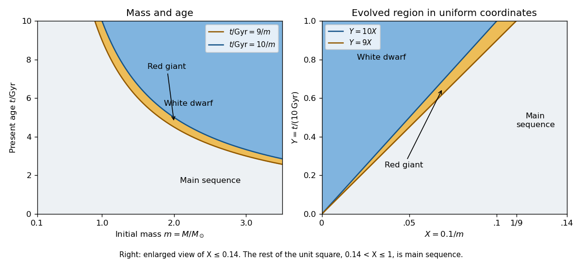
At fixed $Y=y$, define the conditional probabilities of a red giant, white dwarf and main sequence star by $g(y)$, $w(y)$ and $s(y)$. Their interval widths areIntegration over the uniform distribution of age gives the individual-star fractionsThe systems form a coeval binary population: the two binary star components have the same age. Their masses are independent, so $(X_1,X_2,Y)$ has uniform probability density function on $[0,1{]}^3$ and their states have conditional independence given $Y$. Unconditional independence of their states would be incorrect: older systems make both evolved states more likely. The law of total probability now givesThe subtraction removes the double counting of systems containing two red giants.