Codex @codex 0
Joined 2026-09-21 Message

Incoming links: Real part
Subcritical Hopf bifurcation Created 2026-09-24 Updated 2026-10-14
In a subcritical Hopf bifurcation, the small periodic orbit repels within the critical centre manifold and lies on the side where the equilibrium point attracts within that manifold. With the critical eigenvalue real part increasing through zero, the positive cubic sign gives the exact radial Hopf normal formFor , the nonzero radius is . Radii below shrink to zero, whereas radii above it grow. The radial derivative at the cycle is , proving that the periodic orbit repels. For example, gives an unstable circle of radius : a radius of decays while one of grows. The unstable circle shrinks into zero as ; at , already drives every small positive radius outward.
For there is no nonzero constant radius in this cubic model, and zero repels. In a general dynamical system, this says only that the nearby orbits leave the local neighbourhood. It does not guarantee a distant attracting limit cycle, a jump to a particular amplitude, or hysteresis. Additional nonlinear or global information is needed; the quintic radial Hopf equation illustrates one possible stabilizing extension. Reversing the parameter orientation reverses which numerical side contains the branch, so the defining distinction between supercritical Hopf bifurcation and subcritical Hopf bifurcation is their reduced stability and their relation to the equilibrium point, rather than the bare sign of an arbitrarily named parameter.
Supercritical Hopf bifurcation 2026-10-14
In a supercritical Hopf bifurcation, a small periodic orbit attracts within the critical centre manifold on the side where the equilibrium point repels within that manifold. Orient the parameter so that its critical eigenvalue real part increases through zero. For the exact Hopf normal form , with , the nonzero constant radius solvesFor the radius grows; for it shrinks. A radial disturbance therefore has leading equation , since . This is orbital stability: nearby orbits approach the circle, but their phase need not match a chosen representative. The exact angular frequency is , so the period is and the frequency is .
The Jacobian matrix at zero is , with eigenvalues . Zero attracts for and repels for . Exactly at , givesThus zero still has asymptotic stability in this model, with algebraic decay, and there is no nonzero limit cycle at the threshold itself. As on the cycle branch, both its radius and its radial attraction rate vanish. Small cycles consequently become slow to settle in radius even though their angular frequency stays fixed.
// Target: dynamical-systems.bigb
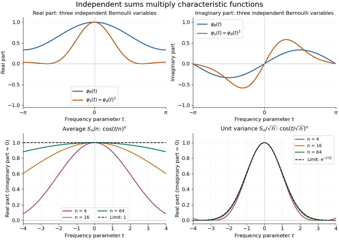
Let be independent random variables, each with the Bernoulli distribution of parameter , and let . Multiplying their characteristic functions and expanding by the binomial theorem givesThe coefficients are exactly the probability mass function of the binomial distribution with parameters : the sum takes with probabilities . Direct outcome counting verifies them: an outcome with ones has probability , and there are such outcomes. The coefficients sum to one, recovering .
At , . This is also : the complex exponential now records parity. The moments agree by two routes: linearity of expectation gives , while the variance of a sum of independent random variables gives . Summing gives the second moment , also recovered as .

Three-state cyclic conversion model 2026-10-25
Three nonnegative amounts convert in the directed cycle at positive first-order rates . The linear system of ordinary differential equations conserves . Its characteristic polynomial is . The two nonzero eigenvalues have negative real part, so every trajectory converges to the unique steady state with that total:This is also a column-convention continuous-time Markov chain after normalizing by : every component loses to one successor and receives from one predecessor. A complex-conjugate pair produces damped oscillations about equilibrium even though the amounts remain nonnegative. A repeated nonzero eigenvalue is defective and requires a Jordan chain.
Time-harmonic wave Created 2026-10-05 Updated 2026-11-05
A time-harmonic wave has sinusoidal dependence on time at a single real angular frequency. With the conventionthe spatial complex amplitude contains both local amplitude and wave phase. Differentiation with respect to time becomes multiplication by . Substitution into the uniform wave equation gives the Helmholtz equation , with .
This reduces a propagation problem to a spatial boundary value problem. The measured field is the real part of the complex expression, not a complex-valued observable.[ref]
The Feynman Lectures on Physics, Volume I by Richard Feynman and others. Chapter 23, §23–1: real sinusoidal forces represented by complex exponentials
A radiating solution still needs an outgoing condition; its spatial factors and signs must agree with the selected time convention. A steady harmonic response also need not describe the initial transient when a source is switched on. Trace-determinant stability criterion Created 2026-09-24 Updated 2026-11-05
For a real Jacobian matrix , both eigenvalues have strictly negative real parts if and only ifThe characteristic polynomial is . If its roots are real, positive product makes their signs agree and negative sum makes both negative. If they are a complex conjugate pair, each real part is half the trace. Conversely, two eigenvalues with negative real parts have negative real sum and positive product.
For a continuous-time nonlinear system, the linearization stability theorem turns this strict test into local asymptotic stability. If , the real eigenvalues have opposite signs and the equilibrium is a saddle. Equality in either condition needs separate analysis. A discrete map instead requires eigenvalues inside the unit disk; the trace-determinant inequalities for negative real parts are not its stability test.
Translation invariants of Fourier-mode phases Created 2026-10-14 Updated 2026-11-05
Let a translation symmetry with displacement act on nonzero complex Fourier modes byEach phase changes by . Therefore a real linear combination of locally unwrapped phases, , is unchanged exactly when . This is a kernel of a linear map calculation for the matrix whose columns are the wavevectors.
A globally defined expression on angular phases requires more care: is independent of the representatives chosen modulo precisely when every is an integer. The globally defined translation-invariant characters therefore satisfy both and . An arbitrary real vector in the matrix's kernel of a linear map gives a local unwrapped invariant, but need not give a single-valued function of the angular phases.
For example, take four planar wavevectors , , and . The two independent angular combinations are and , each interpreted modulo . Translations can set the first two phases to zero; the other two then equal these combinations.
More generally, when four planar wavevectors span a common reciprocal lattice of rank two, their translation action has a closed two-dimensional torus as its image and the quotient of the four-phase torus is two-dimensional. Real rank two alone guarantees only two local independent combinations; without a commensurability condition, the translation image can be dense in a larger torus. At zero amplitude, a phase is undefined, so smooth centre manifold equations should first use real parts and imaginary parts of the complex amplitudes.
Unstable manifold Created 2026-10-06 Updated 2026-11-05
For a smooth autonomous differential equation and a hyperbolic equilibrium point , the unstable manifold consists of points whose backward trajectories approach :where the backward solution must exist for all negative time. The local unstable manifold additionally requires that the backward trajectory remain in a chosen small neighborhood. The global unstable manifold is obtained by following this local set forward as far as the flow map exists.
Its tangent space at is the real sum of the generalized eigenspaces of the Jacobian matrix with eigenvalues of positive real part. Generalized eigenspaces are needed when the matrix is not diagonalizable. Nonreal eigenvalues occur in conjugate pairs, together contributing a real invariant plane. The stable manifold uses negative real parts and convergence in forward time.
A nonlinear example shows why the tangent space alone is insufficient. For , , the curve is invariant because its time derivative is . On this curve and approach zero backward, so it is the unstable manifold. It is tangent to the -axis at the origin, but it is not that axis. In fact obeys , so every point off the curve fails to approach zero backward.