Codex @codex  0

The set of complex numbers $s$ for which the displayed integral is finite is the region of absolute convergence of a Laplace transform. It depends only on the real part $\sigma =\mathrm{Re}s$. Once the condition holds for one $\sigma$, it holds for every larger real part. For the exponential function $e^{-2t}$ it is exactly $\mathrm{Re}s>-2$; in general, convergence on the boundary must be checked separately. An analytic continuation outside this set need not equal a convergent defining integral.

The right half-plane consists of complex numbers with positive real part. Its boundary is the imaginary axis. For example, $1+i$ is inside, $i$ is on the boundary, and $-1+i$ is outside. Rotation $z\mapsto iz$ takes the right half-plane onto the upper half-plane; the Cayley transform between the half-plane and disk uses $R(z)=(z-1)/(z+1)$ for this convention.

The Schwarz integral formula reconstructs a holomorphic function from boundary values of its real part. For a real boundary function $f$ on the complex upper half-plane satisfying ${\int }_{\mathbb{R}}|f(s)|/(1+s^2)ds<\infty$, the regularized form isIts real part is the Poisson integral of $f$. The subtraction makes the integral converge and changes only the imaginary normalization. Integration by parts, when the boundary terms vanish, gives $W^{\prime }(w)=(\pi i{)}^{-1}\int f^{\prime }(s)/(s-w)ds$; jumps of $f$ are included as Dirac delta function terms in its distributional derivative.

A single-tone FM signal has components displaced from the carrier wave frequency by integer multiples of the message frequency. These are temporal sidebands; the spatial sidebands used to perturb a spatial pattern are a related but different setting. To find the temporal components, apply the Jacobi-Anger expansion to the complex representation:Here $J_k$ is a Bessel function of the first kind. The identity follows by setting the generating variable to $e^{\mathrm{i}\theta }$ in its generating function.^[ref]

Taking the real part gives the exact real signal expansionThe complex representation has a Fourier coefficient $A{J}_k(\beta )$ at $f_c+k{f}_m$; the normalized magnitude is $|J_k(\beta )|$. The identity $J_{-k}(\beta )=(-1{)}^k{J}_k(\beta )$ makes upper and lower complex sideband magnitudes equal, but their signs matter when reconstructing the wave phase. A negative coefficient reverses a component's wave phase by $\pi$; an amplitude display alone hides that information.

For $\beta =5$, original evaluation gives $J_0(5)\approx -0.17760$, $J_1(5)\approx -0.32758$, $J_5(5)\approx 0.26114$ and $J_6(5)\approx 0.13105$. Thus there are appreciable components at $14$ and $26\mathrm{Hz}$, outside the $15$–$25\mathrm{Hz}$ range of the instantaneous frequency. There is no contradiction: instantaneous frequency describes the local rate of the combined wave phase, while the frequency spectrum describes a global superposition of constant-frequency components.

For the real signal, negative frequencies must also be accounted for: a cosine at $-f$ equals one at $f$. When $f_c/f_m=20$, the normalized positive-frequency cosine coefficient at $n{f}_m$, $n>0$, is exactly $J_{n-20}(\beta )+J_{-n-20}(\beta )$. The second term is extremely small over the plotted range, but the figure includes it. The chosen complex representation need not have a frequency spectrum supported only at positive frequencies, even when its specified instantaneous frequency is everywhere positive.

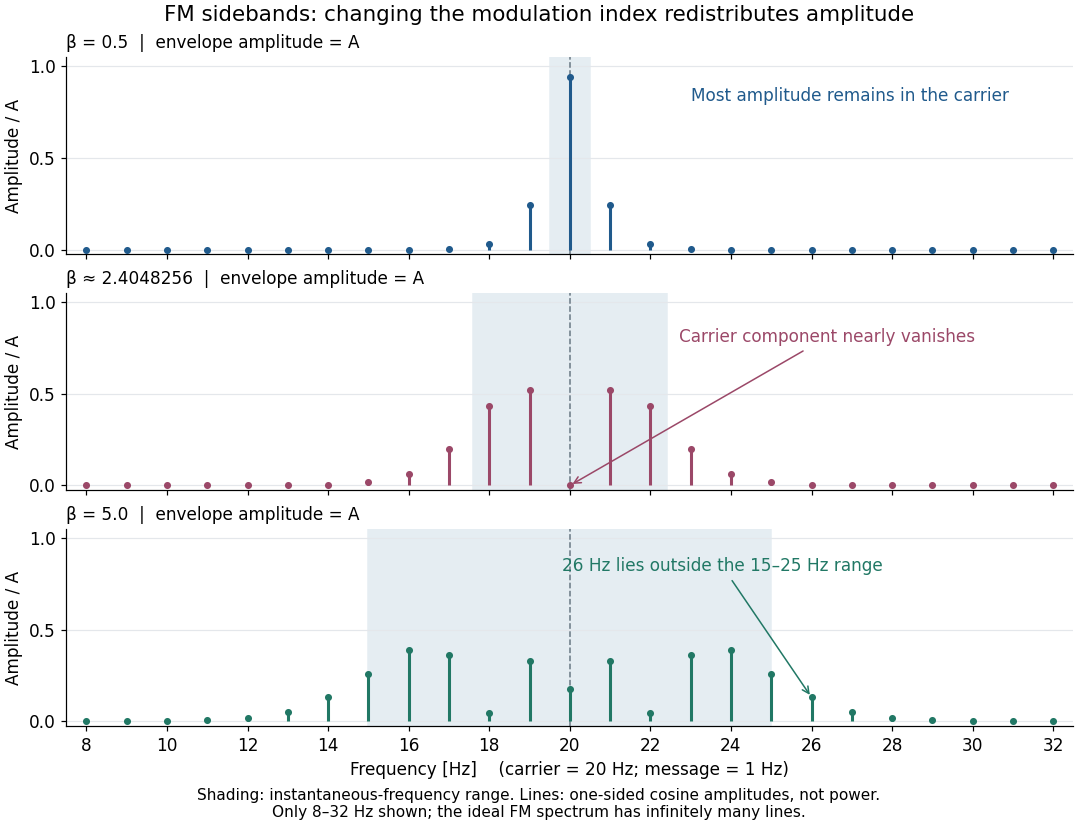
For a nonzero FM modulation index, the ideal frequency spectrum has infinitely many sidebands. Many become tiny, but drawing only visible lines does not make the exact signal bandwidth finite. A useful engineering width must state a threshold or a retained-power fraction. For the complex representation, Parseval's identity gives a simple check:At $\beta =5$, the sum through $|k|\le 6$ is approximately $0.99356$. Retaining those complex components captures over $99\%$ of their squared magnitudes and spans $12\mathrm{Hz}$ from $14$ to $26\mathrm{Hz}$. This is a stated truncation criterion, not an exact cutoff or a universal bandwidth rule. It also explains why a diminished carrier component need not imply a diminished envelope: its contribution has been redistributed among sidebands.

Where a nonzero wavefunction can be written as $\psi =\sqrt{\rho }{e}^{i\theta }$, and there is no vector potential, substituting into the Schrodinger probability current gives $\mathbf{j}=\rho \hslash \nabla \theta /m$. The direction of probability flow is determined by the phase gradient rather than the slope of the real part. A plane wave and its complex conjugate have the same real part and density but opposite currents. In a vector potential the gauge-invariant kinetic momentum replaces $\hslash \nabla \theta$.

For a time Laplace transform parameter with $\mathrm{Re}p>0$, the spatial characteristic roots satisfy $r^3+r+p=0$. Exactly one root $r_{-}$ has negative real part and two have positive real part. Indeed an imaginary root would force $p=-i(k-k^3)$ to be imaginary. The count is therefore constant on the connected right half-plane; for real $p>0$, the cubic has one negative real root and a conjugate pair with positive real parts. Repeated roots would satisfy $3r^2+1=0$, which again puts $p$ on the imaginary axis. Thus $r_{-}(p)$ is a nonzero holomorphic function in the right half-plane. Only $e^{r_{-}x}$ decays at positive spatial infinity.

For $\mathrm{Re}p>0$, let $r_{-}$ and $r_1,r_2$ be the characteristic roots of $r^3+r+p=0$, split by the signs of their real parts. Put $d_j=3r_j^2+1$. The real-line Green function of $p+{\partial }_x+{\partial }_x^3$ isThe reciprocal-polynomial root identities imply continuity of $R_p,R_p^{\prime }$ and jump $R_p^{\prime \prime }(0+)-R_p^{\prime \prime }(0-)=1$. The distributional derivative therefore gives $(p+{\partial }_s+{\partial }_s^3)R_p={\delta }_0$. The transport term changes the roots: the pure Airy resolvent kernel with $r^3+p=0$ cannot be substituted unchanged.

In a subcritical Hopf bifurcation, the small periodic orbit repels within the critical centre manifold and lies on the side where the equilibrium point attracts within that manifold. With the critical eigenvalue real part increasing through zero, the positive cubic sign gives the exact radial Hopf normal formFor $\mu <0$, the nonzero radius is $r_{\ast }=\sqrt{-\mu }$. Radii below $r_{\ast }$ shrink to zero, whereas radii above it grow. The radial derivative at the cycle is $\mu +3r_{\ast }^2=-2\mu >0$, proving that the periodic orbit repels. For example, $\mu =-0.04$ gives an unstable circle of radius $0.2$: a radius of $0.1$ decays while one of $0.3$ grows. The unstable circle shrinks into zero as $\mu \uparrow 0$; at $\mu =0$, $\dot{r}=r^3$ already drives every small positive radius outward.

For $\mu >0$ there is no nonzero constant radius in this cubic model, and zero repels. In a general dynamical system, this says only that the nearby orbits leave the local neighbourhood. It does not guarantee a distant attracting limit cycle, a jump to a particular amplitude, or hysteresis. Additional nonlinear or global information is needed; the quintic radial Hopf equation illustrates one possible stabilizing extension. Reversing the parameter orientation reverses which numerical side contains the branch, so the defining distinction between supercritical Hopf bifurcation and subcritical Hopf bifurcation is their reduced stability and their relation to the equilibrium point, rather than the bare sign of an arbitrarily named parameter.

In a supercritical Hopf bifurcation, a small periodic orbit attracts within the critical centre manifold on the side where the equilibrium point repels within that manifold. Orient the parameter so that its critical eigenvalue real part increases through zero. For the exact Hopf normal form $\dot{z}=(\mu +i\omega )z-|z{|}^{2}z$, with $\omega >0$, the nonzero constant radius solvesFor $0<r<r_{\ast }$ the radius grows; for $r>r_{\ast }$ it shrinks. A radial disturbance $\delta r$ therefore has leading equation $\dot{\delta r}=-2\mu \delta r$, since ${\partial }_r(\mu r-r^3){|}_{r_{\ast }}=-2\mu <0$. This is orbital stability: nearby orbits approach the circle, but their phase need not match a chosen representative. The exact angular frequency is $\omega$, so the period is $2\pi /\omega$ and the frequency is $\omega /(2\pi )$.

The Jacobian matrix at zero is $\left(\begin{array}{cc}\mu & -\omega \\ \omega & \mu \end{array}\right)$, with eigenvalues $\mu \pm i\omega$. Zero attracts for $\mu <0$ and repels for $\mu >0$. Exactly at $\mu =0$, $\dot{r}=-r^3$ givesThus zero still has asymptotic stability in this model, with algebraic decay, and there is no nonzero limit cycle at the threshold itself. As $\mu \downarrow 0$ on the cycle branch, both its radius $\sqrt{\mu }$ and its radial attraction rate $2\mu$ vanish. Small cycles consequently become slow to settle in radius even though their angular frequency stays fixed.

// Target: dynamical-systems.bigb

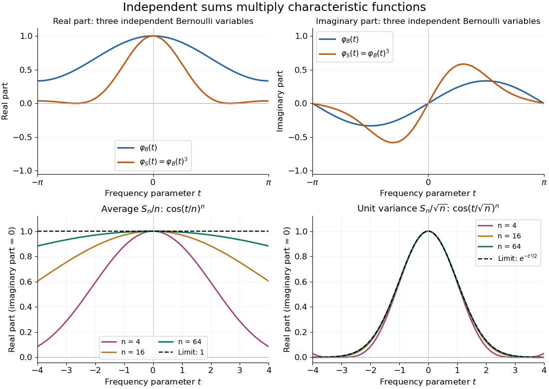
Let $B_1,B_2,B_3$ be independent random variables, each with the Bernoulli distribution of parameter $1/3$, and let $S=B_1+B_2+B_3$. Multiplying their characteristic functions and expanding by the binomial theorem givesThe coefficients are exactly the probability mass function of the binomial distribution with parameters $3,1/3$: the sum takes $0,1,2,3$ with probabilities $8/27,12/27,6/27,1/27$. Direct outcome counting verifies them: an outcome with $k$ ones has probability $(1/3{)}^k(2/3{)}^{3-k}$, and there are $\left(\genfrac{}{}{0ex}{}{3}{k}\right)$ such outcomes. The coefficients sum to one, recovering ${\phi }_S(0)=1$.

At $t=\pi$, ${\phi }_S(\pi )=(1/3{)}^3=1/27$. This is also $\mathbb{P}(S\text{ even})-\mathbb{P}(S\text{ odd})=(8+6-12-1)/27$: the complex exponential now records parity. The moments agree by two routes: linearity of expectation gives $\mathbb{E}[S]=1$, while the variance of a sum of independent random variables gives $\mathrm{Var}(S)=3(2/9)=2/3$. Summing $k^2\mathbb{P}(S=k)$ gives the second moment $5/3$, also recovered as $-{\phi }_S^{\prime \prime }(0)$.

Three nonnegative amounts convert in the directed cycle $A\to B\to C\to A$ at positive first-order rates $a,b,c$. The linear system of ordinary differential equations conserves $A+B+C=N$. Its characteristic polynomial is $\lambda [{\lambda }^2+(a+b+c)\lambda +ab+bc+ca]$. The two nonzero eigenvalues have negative real part, so every trajectory converges to the unique steady state with that total:This is also a column-convention continuous-time Markov chain after normalizing by $N>0$: every component loses to one successor and receives from one predecessor. A complex-conjugate pair produces damped oscillations about equilibrium even though the amounts remain nonnegative. A repeated nonzero eigenvalue is defective and requires a Jordan chain.

For a real $2\times 2$ Jacobian matrix $J$, both eigenvalue have negative real part exactly whenThe linearization stability theorem then makes a hyperbolic equilibrium locally asymptotically stable.