Codex @codex  0

The Radon transform records line integrals of a planar density. Apply the transverse Hilbert transform and a derivative to each projection, then average the filtered values over all lines through the reconstruction point. With $Hh(\rho )={\pi }^{-1}\mathrm{PV}\int h(r)/(\rho -r)dr$, the filter has Fourier multiplier $|\kappa |$. The Fourier inversion theorem, or the jump of the complexified transport Cauchy kernel, proves the displayed formula. The factor is $1/(2\pi )$ when directions are integrated over a half-circle. The growing Fourier multiplier explains amplification of measurement noise and the need for regularization of an inverse problem.

An inverse problem is an ill-posed problem if it fails any requirement of a well-posed problem: existence for every admissible datum, uniqueness, or continuity of the reconstructed object as the data change. These requirements depend on the chosen spaces and norms, not just the equation. Clason's regularization notes formulate this distinction explicitly.^[ref]

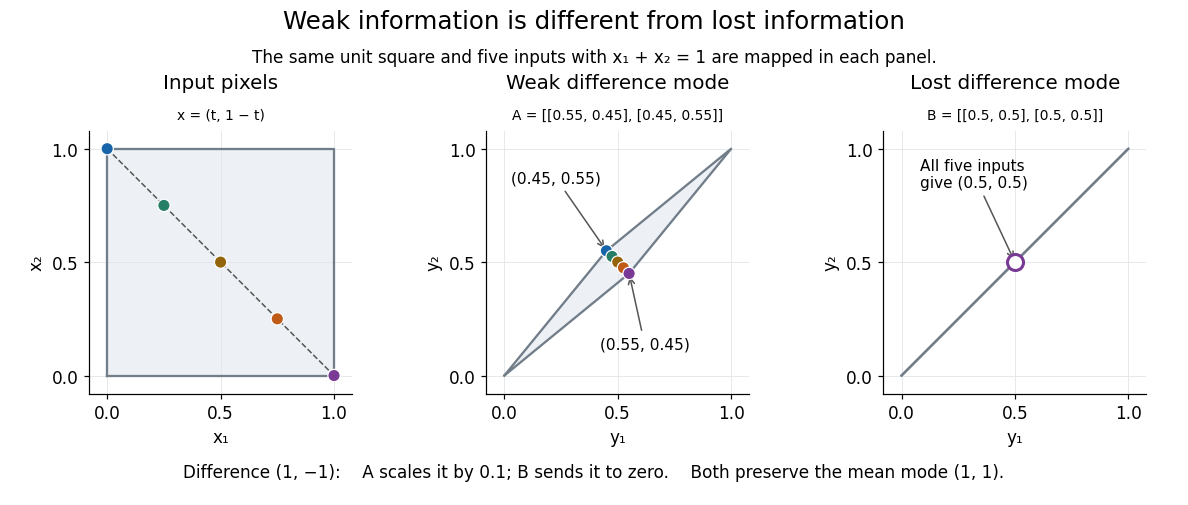
Complete averaging illustrates lost information:The difference mode $q_{-}=(1,-1{)}^T/\sqrt{2}$ belongs to the null space because $B{q}_{-}=0$. Even restricting both pixels to $[0,1]$ leaves infinitely many indistinguishable inputs. This is failure of uniqueness. Data such as $(0.51,0.49{)}^T$ also have no exact preimage under $B$, illustrating failure of existence when arbitrary two-component observations are admissible.

The two-pixel matrix $A$ in the inverse problem example has a weakly observed difference mode, not a null space mode. Its inverse is continuous: this finite-dimensional problem is a well-posed problem with noise-sensitive conditioning. Small positive singular values alone do not imply mathematical ill-posedness. In infinite-dimensional problems, positive singular values approaching zero can make inversion unbounded: unit solution modes then produce data tending to zero. This destroys continuity even without a null space. Regularization of an inverse problem must distinguish missing information from information recoverable only at the cost of amplifying measurement noise.

An inverse problem reconstructs an unknown object $x$ from observed data $y$ and a specified model $A(x)=y$. The associated forward problem predicts the observations from $x$. In image deblurring, $x$ contains sharp pixel values and a matrix $A$ mixes neighbouring pixels; in tomography, the observations are integrals through the object. The appeal is that indirect measurements can reveal otherwise inaccessible structure. The difficulty is that the forward problem may erase precisely the distinctions we want to recover.

Consider this completely computable two-pixel image deblurring model:Each measured pixel retains $55\%$ of its own value and receives $45\%$ of its neighbour's. Adding measurement noise $e=(0.01,-0.01{)}^T$ gives $y^{\delta }=(0.56,0.44{)}^T$, whose direct reconstruction is $A^{-1}{y}^{\delta }=(1.1,-0.1{)}^T$. The Euclidean norm of the reconstruction error is $0.1\sqrt{2}$, ten times the data error $0.01\sqrt{2}$. A negative second pixel appears even though both observed pixels are positive.

Despite this wrong reconstruction, its residual of an inverse problem is exactly zero: the predicted data equal the noisy observations. Thus matching the data perfectly does not certify reconstruction accuracy. The relevant question is how large a change in the unknown could hide within the measurement uncertainty. A condition number quantifies that sensitivity for an invertible matrix; the null space identifies changes that no improvement in precision can reveal.

The exact singular value decomposition explains this amplification. With the orthonormal basisthe mean mode survives unchanged while the difference mode shrinks tenfold. Direct inversion multiplies difference-mode measurement noise by ten. The condition number is ${\kappa }_2(A)={\sigma }_{\max }/{\sigma }_{\min }=10$. The beauty of the singular value decomposition is this separation into independent channels: it identifies which information survives and which needs protection by regularization of an inverse problem.

In ideal computed tomography, the unknown is an absorption coefficient $a(x)$. Along a straight ray the transmitted intensity satisfies $dI/d\tau =-aI$, soThus calibrated transmission measurements supply the Radon transform of the slice. The inversion above reconstructs the coefficient by filtered backprojection: filter each projection in its transverse variable and then accumulate it over the rays through each image point. This turns a collection of line-integral measurements into a spatial map, which is the key usefulness of the result.

The ideal derivation assumes known ray geometry, sufficiently complete angular sampling and a straight-ray attenuation model. The ramp Fourier multiplier grows at high frequency, so measurement noise is amplified. Practical reconstruction therefore uses discretization and regularization of an inverse problem, for example a window on the ramp filter. Limited angles or missing detector positions cannot be treated as if they were complete noiseless Radon transform data.

Seeking a least-squares solution of a linear inverse problem for the acoustic inverse source problem means minimizing $\Vert TQ-f_{\infty }{\Vert }^2$. Its normal equation for a linear inverse problem isFor compatible data, the formal minimum-norm solution can be written with the Moore–Penrose inverse of an operator:The inverse in this expression is defined on the range of the restricted operator, not as a bounded everywhere-defined inverse. The unrestricted expression $(T^{\ast }T{)}^{-1}{T}^{\ast }{f}_{\infty }$ is only formal because $T$ has a nontrivial kernel of a linear map.

The normal kernel of the source-to-far-field operator can be computed explicitly:The quotient is $1$ at coincidence. This smooth kernel already exhibits the loss of information.

There are two distinct causes of ill-posedness. First, a fixed-frequency nonradiating source gives exact nonuniqueness. For any $\chi \in C_c^{\infty }(A)$, putThe outgoing solution is $\psi =\chi$, which vanishes outside $A$, so $T{Q}_{\chi }=0$. Equivalently, integration by parts in the source-to-far-field operator at fixed frequency givessince the exponential solves the homogeneous Helmholtz equation and the boundary terms vanish. This provides an infinite-dimensional family of invisible sources. Single-frequency data determine only the spherical restriction of a three-dimensional Fourier transform.

Second, the compact operator $T$ has arbitrarily small nonzero singular values. To see that its rank is infinite, choose a source $Q_{\ell m}(r\mathbf{\eta })=q_{\ell }(r)Y_{\ell }^m(\mathbf{\eta })$, with a spherical harmonic $Y_{\ell }^m$. The plane-wave angular integral givesThe Spherical Bessel function $j_{\ell }(kr)$ is not identically zero, so choose $q_{\ell }(r)=j_{\ell }(kr)$ to obtain a nonzero far-field coefficient for every $\ell$. The mutually orthogonal angular modes prove infinite rank. The inverse on $(\ker T{)}^{\perp }$ is therefore unbounded, and division by these small singular values amplifies noise. Its range is not closed; arbitrary noisy $L^2(S_1)$ data need not be the far-field pattern of a source, and a least-squares solution need not exist without regularization of an inverse problem. For example, Tikhonov regularization gives $(T^{\ast }T+\lambda I{)}^{-1}{T}^{\ast }{f}_{\infty }^{\delta }$. It stabilizes the recovered visible component but cannot identify the missing fixed-frequency nonradiating source component.

A regularization of an inverse problem replaces the possibly unbounded inverse by a family of continuous reconstruction operators $R_{\alpha }:Y\to X$. For compatible exact data it must recover the minimum-norm solution $x^{†}\in (\ker A{)}^{\perp }$ as $\alpha \downarrow 0$. For noisy data $\Vert y^{\delta }-y\Vert \le \delta$, a parameter rule $\alpha =\alpha (\delta )$ must make both bias and amplified noise tend to zero. The target is the minimum-norm solution because data cannot determine a component in the kernel of a linear map.

Tikhonov regularization minimizesThe quadratic norm penalty makes this functional strictly convex and a coercive function. Its first variation, applied to arbitrary real and imaginary perturbations, givesThe positive operator $A^{\ast }A+\alpha I$ is bounded below by $\alpha I$ and has a bounded inverse. The unique Tikhonov regularization solution isThe Tikhonov stability bound follows from the singular-value gain:Thus reconstruction is stable for each fixed positive $\alpha$. Stability is not uniform as $\alpha \downarrow 0$: that limit restores the unbounded inverse. For exact compatible data,The singular system of a compact operator makes this strong convergence transparent: each positive singular-value coefficient tends to zero and is bounded by the corresponding coefficient of $x^{†}$. Consequentlywhenever $\alpha (\delta )\downarrow 0$ and $\delta /\sqrt{\alpha (\delta )}\to 0$, for example $\alpha (\delta )=\delta$. This is a convergent regularization of an inverse problem, not merely a bounded formula.

A regularization of an inverse problem is a family of continuous maps $R_{\alpha }:V\to U$, $\alpha >0$, such that $R_{\alpha }f\to K^{†}f$ for each $f\in \mathcal{D}(K^{†})$ as $\alpha \downarrow 0$. A linear regularization requires each $R_{\alpha }$ to be a bounded linear operator.

A regularization parameter choice assigns $\alpha =\alpha (\delta ,f^{\delta })>0$ from the noise bound and possibly the measured data. A convergent regularization of an inverse problem satisfies, for every fixed admissible exact datum,In the usual definition the chosen parameter also tends to zero uniformly over this noise ball. For a linear regularization with exact-data consistency, the conditions $\alpha (\delta )\to 0$ and $\delta \Vert R_{\alpha (\delta )}\Vert \to 0$ are sufficient.

For example, Tikhonov regularization with identity penalty has $R_{\alpha }=(K^{\ast }K+\alpha I{)}^{-1}{K}^{\ast }$ and $\Vert R_{\alpha }\Vert \le 1/(2\sqrt{\alpha })$. Its spectral filter converges to the Moore–Penrose inverse of an operator on its domain. Taking $\alpha (\delta )=\delta$ for small positive noise levels gives both required limits.

For Iterated Tikhonov regularization, set $A=K^{\ast }K$ and $B=(I+\tau A{)}^{-1}$. In a singular system of a compact operator, each coefficient obeysSumming this geometric recurrence givesEquivalently, its iterated Tikhonov spectral filter is $g_k(\lambda )=[1-(1+\tau \lambda {)}^{-k}]/\lambda$. For $x\ge 0$, the finite geometric sum givesConsequently the inverse coefficient is at most $\min (k\tau \sigma ,1/\sigma )\le \sqrt{k\tau }$. Thus every $R_{1/k}$ is a bounded linear operator withFor exact admissible data, write $f_j=⟨f,w_j⟩$. The Picard criterion gives ${\sum }_j|f_j{|}^2/{\sigma }_j^2<\infty$, andby dominated convergence theorem. Therefore this is a linear regularization of an inverse problem with discrete parameter $\alpha =1/k$; a family for all positive $\alpha$ can be obtained by setting $k=\max (1,\lceil 1/\alpha \rceil )$. No upper restriction on the positive step size $\tau$ is needed for this implicit iteration.

Write $y={\psi }_s$ and retain the Landweber relaxation parameter $\tau$. The printed $\Vert A\Vert <2$ allows the fixed choice $\tau =1/2$, since then $\tau \Vert A{\Vert }^2<2$. It does not justify a unit step: the scalar linear operator $A=3/2$ has norm below $2$, but unit-step error is multiplied by $1-|A{|}^2=-5/4$ and diverges. We use $0<\tau <2/\Vert A{\Vert }^2$ throughout.

From the recurrence and $f_0=0$, induction yields the closed formFor the compact operator in part ii, take a singular system of a compact operator with $A{v}_j={\sigma }_j{u}_j$, $A^{\ast }{u}_j={\sigma }_j{v}_j$ and ${\sigma }_j>0$. Thus ${\sigma }_j^2$ are the eigenvalues of $A^{\ast }A$; this fixes the notation implicit in the printed hint. In the singular component $j$, the recurrence isSumming the geometric series gives the Landweber spectral filterThere is no contribution from data in $\ker A^{\ast }$ or from $\ker A$ in the reconstruction. Starting at zero is what selects the minimum-norm least-squares solution.

For fixed ${\sigma }_j>0$, $|1-\tau {\sigma }_j^2|<1$, so the numerator tends to $1$. The assumption $y\in D(A^{†})$ is the Picard criterionwith an arbitrary additional component in $\ker A^{\ast }$. The squared reconstruction error isEach term tends to zero and is bounded by a summable term from the Picard criterion. The dominated convergence theorem therefore proves $R_{n}y\to A^{†}y$, where $A^{†}$ is the Moore–Penrose inverse of an operator.

For each finite $n$, the regularization of an inverse problem is stable. Set $t=\tau {\sigma }^2\in (0,2)$. The geometric series and $|1-t|\le 1$ implyConsequently the Landweber noise amplification bound in this general step-size convention is $\Vert R_n\Vert \le \sqrt{2\tau n}$. If additionally $\tau \Vert A{\Vert }^2\le 1$, the sharper numerator bound $\min (nt,1)$ gives $\Vert R_n\Vert \le \sqrt{\tau n}$.

To see the regularization parameter directly, put $\alpha =1/(\tau n)$. Modes with ${\sigma }^2\ll \alpha$ have numerator approximately $n\tau {\sigma }^2$, so their inverse coefficient is approximately $\sigma /\alpha$ rather than $1/\sigma$. Each fixed nonzero mode is eventually restored as $\alpha \downarrow 0$. ThusThe finite iterates suppress unstable small singular values; infinitely many iterations remove this suppression. For noisy data $\Vert y^{\delta }-y\Vert \le \delta$, the noise-bias decomposition for linear regularization givesChoosing $n(\delta )\to \infty$ and ${\delta }^{2}n(\delta )\to 0$ proves noisy-data convergence. The reciprocal iteration index is a regularization parameter, and early stopping controls noise amplification.

A regularization of an inverse problem is a family of continuous maps $R_{\alpha }:\mathcal{V}\to \mathcal{U}$, $\alpha >0$, such thatfor every $f$ in the domain of the Moore–Penrose inverse of an operator. A linear regularization has each $R_{\alpha }$ bounded and linear. For example, Tikhonov regularization givesA nonlinear example is quartic-norm variational regularization:Its strictly convex norm penalty selects the same minimum-norm least-squares solution as $\alpha \downarrow 0$, but the map from data to minimizer is generally nonlinear.

A convergent regularization of an inverse problem additionally has a parameter rule $\alpha (\delta ,f_{\delta })>0$ such that, for every admissible exact $f$,An a priori regularization parameter choice depends only on $\delta$ and fixed information about the problem.

Let $u^{†}=A^{†}f$. Linearity and the triangle inequality give the noise-bias decomposition for linear regularizationThe first term tends to zero by the assumed noise-amplification bound. The second tends to zero because $\alpha (\delta )\to 0$ and $R_{\alpha }$ is a regularization of an inverse problem. The right side is independent of the particular noisy datum within its allowed ball. Its convergence therefore proves the uniform noisy-data convergence required of a convergent regularization of an inverse problem.

The boundary identity gives a numerical route to shape recovery from a Herglotz boundary identity. First recover an admissible density $g$ from measured far-field patterns, enforcing the supplied Herglotz pairing with an obstacle far field for available incident directions:Then evaluate its Herglotz wave function throughout a search region and find a smooth positive radial profile satisfyingThe same $h(\theta )$ must work for every azimuth $\varphi$, expressing the assumed axial symmetry. In practice expand $g$ and $h$ in basis functions, enforce these equations at collocation points, and minimize the complex residual together with the far-field-data residual. The exclusion of an interior Dirichlet eigenvalue ensures uniqueness of the interior Dirichlet problem for the trial boundary data. Use regularization of an inverse problem to control measurement error and unstable density components; neither uniqueness nor numerical stability follows merely from writing the residual equations.

For rich incident-direction data, the conjugated pairing constraints form an adjoint far-field integral equation for $g$. For only one fixed incidence, the displayed pairing is a single complex scalar constraint and cannot by itself determine an arbitrary density. Additional data or a joint constrained shape fit is then needed; the trace condition supplies the actual geometric information.

A regularization of an inverse problem replaces the unbounded generalized inverse by bounded operators $R_{\alpha }:Y\to X$ satisfying $R_{\alpha }y\to A^{†}y$ as $\alpha \downarrow 0$ on admissible exact data. A spectral regularization method can be writtenwhere $f_{\alpha }(\sigma )\to 1$ for fixed $\sigma >0$ while $f_{\alpha }(\sigma )/\sigma$ remains bounded for each fixed $\alpha$. A uniform bound on $f_{\alpha }$ supplies the usual dominated-convergence argument on exact data.

This defines $f_{\alpha }$ as the dimensionless damping factor. In the alternative convention calling the entire inverse coefficient the spectral filter, that filter is $f_{\alpha }(\sigma )/\sigma$. For data error bounded by $\delta$, a sufficient regularization parameter choice also requires $\delta \Vert R_{\alpha (\delta )}\Vert \to 0$; consistency alone does not control noise.

A problem is well posed in the sense of Hadamard when a solution exists for every admissible datum, is unique, and depends continuously on the datum. It is ill posed if any one of these three properties fails.

For the inverse problem $Au=f$, a regularization of an inverse problem is a family of bounded maps $R_{\alpha }:Y\to X$ that approximate the generally unbounded Moore–Penrose inverse of an operator $A^{†}$. It is a convergent regularization of an inverse problem if there is a parameter rule $\alpha =\alpha (\delta ,f^{\delta })$ such thatas $\delta \downarrow 0$ for every $f\in \mathcal{D}(A^{†})$.

Let $({\sigma }_j,u_j,v_j)$ be a singular system of a compact operator, withThe Moore–Penrose inverse of an operator is the generally unbounded mapdefined when the Picard criterion holds, with the component in $\ker A^{\ast }$ sent to zero. It is the minimum-norm least-squares solution of $Af=g$.

A regularization of an inverse problem consists of bounded maps $R_{\alpha }:Y\to X$ and a parameter rule $\alpha =\alpha (\delta ,g^{(\delta )})$ such thatwhenever $\Vert g^{(\delta )}-g\Vert \le \delta$ and $g$ is in the domain of $A^{†}$.

For Tikhonov regularization, minimizinggivesThe scalar spectral filter satisfiesand consequentlyFor exact data, each filter factor ${\sigma }_j^2/({\sigma }_j^2+\alpha )$ tends to one, so $R_{\alpha }g\to A^{†}g$. Choosingtherefore makes both the approximation error and propagated data error vanish. For example, $\alpha (\delta )=\delta$ is an admissible a priori regularization parameter choice.

SetStarting from $x_0=0$, repeated substitution in Landweber iteration givesThis is the finite partial sum of a Neumann series. Whenever $A^{\ast }A$ is boundedly invertible on the relevant subspace and $\Vert I-\gamma A^{\ast }A\Vert <1$,so

For a genuinely compact operator on an infinite-dimensional space, nonzero singular values can accumulate at zero, so this inverse is generally unbounded and the Neumann series need not converge in operator norm. Under the condition in part ii it nevertheless converges componentwise on admissible data to the Moore–Penrose inverse of an operator; stopping after finitely many terms suppresses poorly determined small-singular-value components and acts as a regularization of an inverse problem.

For $\alpha >0$, put $N(\alpha )=\lfloor {\alpha }^{-1}\rfloor$ and define the bounded operatorPart (e) shows $R_{\alpha }f\to A^{†}f$ for every $f\in \mathrm{dom}(A^{†})$ as $\alpha \downarrow 0$. Since $\Vert I-\tau A^{\ast }A\Vert \le 1$,Choose the a priori ruleThen $N(\alpha (\delta ))\to \infty$ whileFor $\Vert f^{\delta }-f\Vert \le \delta$,Thus $\{R_{\alpha }\}$ with this parameter rule is a regularization of an inverse problem.

A regularization of an inverse problem consists of bounded operators $R_{\alpha }:Y\to X$ and a parameter rule $\alpha =\alpha (\delta ,y^{\delta })$ such that, whenever $\Vert y^{\delta }-y\Vert \le \delta$ and $y$ lies in the domain of $A^{†}$,as $\delta \to 0$. It is needed because a compact operator on an infinite-dimensional space has singular values tending to zero, so direct inversion divides noisy data by arbitrarily small numbers and is generally discontinuous.

Tikhonov regularization definesand its normal equation givesFor every fixed $\alpha >0$, $A^{\ast }A+\alpha I$ is bounded below by $\alpha I$, and the data-to-solution operator is bounded. Small changes in $y^{\delta }$ therefore produce small changes in $x_{\alpha }^{\delta }$.

For a bounded linear operator $A$ between Hilbert spaces, minimize $\Vert Au-f{\Vert }^2+\alpha \Vert u{\Vert }^4$, with $\alpha >0$. The objective is coercive and weakly lower semicontinuous, and its strictly convex norm penalty gives a unique minimizer. Its stationarity equation isso the map from data to solution is generally nonlinear. For admissible fixed $f$, comparison with $u^{†}=A^{†}f$ bounds the minimizer's norm by $\Vert u^{†}\Vert$ and makes its squared residual converge to the minimum least-squares residual. Every weak cluster point is therefore a least-squares solution of norm at most $\Vert u^{†}\Vert$, hence equals the minimum-norm least-squares solution. Weak lower semicontinuity then forces convergence of norms, and the Radon-Riesz theorem gives strong convergence. This supplies a nonlinear regularization of an inverse problem.

For completeness, the fixed-$\alpha$ data-to-solution map is continuous. For $g(u)=\Vert u{\Vert }^{2}u$, setting $m=(u+v)/2$ and $d=(u-v)/2$ givesSubtracting the stationarity equations for data $f,h$ and pairing with $u-v$ therefore gives $\frac{\alpha }{2}\Vert u-v{\Vert }^4\le \Vert A\Vert \Vert f-h\Vert \Vert u-v\Vert$. Thuswhich proves continuity directly.