Richardson-Dushman law ($J=A{T}^2\exp [-W/(k_{B}T)]$)

The Richardson-Dushman law models the magnitude of emitted electric current density asHere $T$ is absolute thermodynamic temperature, $W$ is the work function, $k_B$ is the Boltzmann constant, and $A$ is the Thermionic Richardson constant. The signed electric current density points opposite to the outgoing Electron motion; $J$ here is positive. For uniform emission over area $S$, the emitted electric current magnitude is $I=SJ$.

The Richardson-Dushman law assumes an emitter close to thermal equilibrium, a surface with a well-defined and approximately constant work function over the fitted temperature range, and predominantly thermal escape over the barrier. Interpreting a measured collector electric current with this law additionally requires an emission-limited thermionic current, known emitting area, and negligible return emission from the collector. Strong electric fields can lower the surface barrier or enable quantum tunnelling; then this zero-field expression is insufficient.

For a deliberately chosen teaching model, take $W=2.0\mathrm{eV}$ and $A=120\mathrm{A}\mathrm{c}{\mathrm{m}}^{-2}{\mathrm{K}}^{-2}$, expressing the barrier in electronvolts. These are illustrative parameters, not measured properties of a named material. Using $k_B=8.617333262\times 10^{-5}\mathrm{eV}{\mathrm{K}}^{-1}$, at $1000\mathrm{K}$ the Boltzmann factor is about $8.33\times 10^{-11}$, yetA 20 percent increase in temperature raises the predicted electric current density by about 69 times. For a chosen emitting area $S=0.010\mathrm{c}{\mathrm{m}}^2$, these correspond to approximately $0.100\mathrm{mA}$ and $6.89\mathrm{mA}$ if collection is complete. The small escaping fraction is replenished by the external electrical circuit.

The sensitivity is especially clear from the logarithmic derivative at fixed $A,W$:In the chosen model at $1000\mathrm{K}$, a $1\mathrm{K}$ rise changes $J$ by about 2.5 percent to first order. Accurate temperature measurement matters even when electric current measurement is easy.

The coefficient $A$ has dimensions of electric current density divided by squared temperature. For ideal nonrelativistic particles with the free electron mass, two spin states, a planar uniform surface, and unit escape transmission, the thermionic tail-flux derivation giveswhere $e$ is the positive elementary charge and $h$ is the Planck constant. The two area units differ by a factor of $10^4$. A fitted $A$ need not equal $A_0$: reflection at the surface, the electronic band structure, and uncertain emitting area affect the inferred coefficient. A constant escape transmission $\tau$ would give $A=\tau A_0$ in this simple model; an energy-dependent transmission generally requires an integral instead.

The name joins Owen Willans Richardson with Saul Dushman. Dushman's 1923 paper develops a thermodynamic treatment of Electron emission analogous to evaporation and evaluates the prefactor using quantum ideas.^[ref]

Choose a fixed positive reference $A_{\mathrm{ref}}$ with the same units as $A$. Taking the natural logarithm of a dimensionless ratio givesThus the Richardson plot is a straight line when $A$ and $W$ are constant, with slope $-W/k_B$ and intercept $\ln (A/A_{\mathrm{ref}})$. The familiar notation $\ln (J/T^2)$ silently chooses units; the reference makes that choice explicit. Changing $A_{\mathrm{ref}}$ shifts the intercept and leaves the inferred work function unchanged. If the horizontal axis instead uses $1000\mathrm{K}/T$, its slope is $-W/(1000\mathrm{K}{k}_B)$.

For the chosen $2.0\mathrm{eV}$ example, choose $A_{\mathrm{ref}}=120\mathrm{A}\mathrm{c}{\mathrm{m}}^{-2}{\mathrm{K}}^{-2}$. Then $y(1000\mathrm{K})=-23.2090$ and $y(1200\mathrm{K})=-19.3409$. Their slope is approximately $-23209\mathrm{K}$, giving $W=2.0\mathrm{eV}$. Two temperatures determine a line algebraically; several temperatures allow curvature and drift to be detected. These values are calculated, rather than experimental observations.

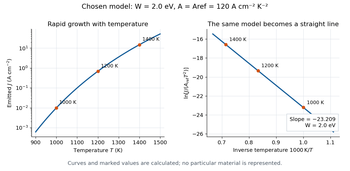
A straight trace alone does not establish a unique surface work function. Adsorption, changing surface coverage, or a mixture of regions with different barriers can change the inferred slope. For independent emitting patches with area fractions $f_i$, constant $A_i$ and barriers $W_i$,Lower barriers contribute disproportionately. Even with fixed patches, the slope of the Richardson plot gives a temperature-dependent weighted mean of the $W_i$, rather than their simple area average. If $A$ or $W$ themselves vary with temperature, the apparent slope-derived barrier becomesCheck collection, temperature calibration, and surface stability before assigning curvature to a new emission mechanism.

Consider a planar surface with outward normal along $z$. For an auxiliary equilibrium electron gas just outside it, let $n_v$ be the total number density, counting both signs of $v_z$. Its Maxwell-Boltzmann velocity distribution has normal-component densityAn Electron with $v_z>0$ crosses more area per unit time when it moves faster. The outgoing number flux therefore uses $v_z{f}_z$, rather than just the probability of $v_z>0$:This integral contributes only $T^{1/2}$. Holding a classical bulk number density fixed and imposing a normal kinetic energy threshold $W$ would instead give $\Gamma =n\sqrt{k_{B}T/(2\pi m_e)}{e}^{-W/(k_{B}T)}$; that argument alone does not produce $T^2$.

For the ideal surface model, measure external Electron energies from the metal's chemical potential $\mu$. A freely propagating external state has $E-\mu =W+p^2/(2m_e)$. When $W\gg k_{B}T$, its Fermi-Dirac distribution reduces to the Maxwell–Boltzmann statistics tail. Counting two spin states per phase space cell of volume $h^3$ givesEach of the three Gaussian integrals supplies $T^{1/2}$. Combining this $T^{3/2}$ state count with the $T^{1/2}$ crossing factor givesThe auxiliary atmosphere supplies an equilibrium state-counting argument; an operating collector removes the outgoing Electrons. It need not maintain a real equilibrium gas throughout the gap. Unit transmission and the ideal free Electron state count are substantive assumptions, so this calculation does not determine an arbitrary real surface's measured $A$.

In particular, Electrons inside a metal generally form a degenerate Fermi gas. A classical distribution for the escaping tail does not imply a classical distribution for the whole interior. Richardson himself emphasized this distinction in his lecture.^[ref]