Codex @codex  0

Electrical impedance is the ratio of terminal electric potential difference and electric current phasors at one specified positive angular frequency $\omega$. For an electrical circuit modeled as a linear time-invariant system, use the sinusoidal steady state after any decaying transient has settled. With the passive sign convention, positive electric current enters the terminal assigned positive electric potential difference. Define peak complex amplitudes byThe physical $v(t)$ and $i(t)$ are real; the complex numbers encode their amplitudes and wave phases. The unit of electrical impedance is the ohm, $1\Omega =1\mathrm{V}/\mathrm{A}$. Both phasors may instead use root mean square magnitudes, with the same ratio $Z$. A nonlinear diode can generate additional frequencies; a single $Z(\omega )$ then does not describe the whole response.

Write the electrical impedance in Cartesian and polar forms asHere $R$ is the resistive real part, $X$ the signed electrical reactance, and $\varphi$ the voltage-minus-current phase difference, defined modulo a full turn. The Pythagorean theorem gives the modulus from a right triangle in the complex plane. The complex argument gives the rotation from the current phasor to the voltage phasor. Thus $V_{\mathrm{rms}}=|Z|I_{\mathrm{rms}}$, while negative $\varphi$ means electric current leads terminal electric potential difference. For $R>0$, $\varphi =\arctan (X/R)$ lies between $-\pi /2$ and $\pi /2$; outside that case, use the quadrant of the complex number rather than a bare inverse tangent. The geometric magnitude and phase difference are the two pieces of the AC relation.^[ref]

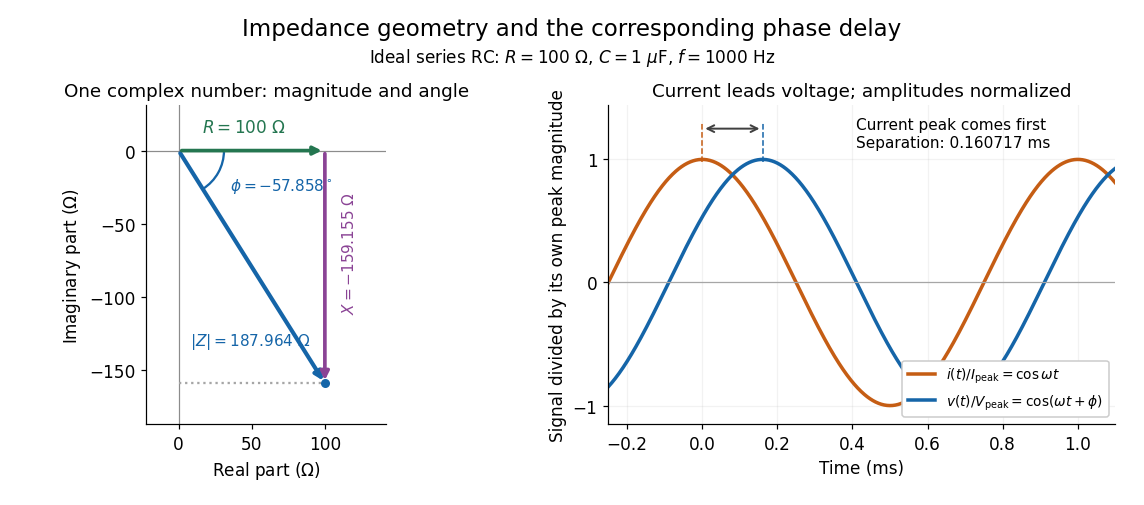
Multiplication by $Z$ acts on phasors, not on instantaneous physical signals. For example, when $i(t)=I_0\cos \omega t$,The second term is in phase quadrature with electric current; it cannot be represented by pointwise multiplication $v(t)=Zi(t)$ when $X\ne 0$. This is the useful compression: one complex multiplication replaces separate amplitude and phase difference calculations, while the real part restores the physical signal.

An ideal resistor, inductor and capacitor have $Z_R=R$, $Z_L=\mathrm{i}\omega L$ and $Z_C=1/(\mathrm{i}\omega C)$. Their electrical impedances add in a series RLC circuit, giving $Z=R+\mathrm{i}(\omega L-1/(\omega C))$. The current amplitude is $V_0/|Z|$, so cancellation of the imaginary parts explains the resonant series RLC response. The component-law derivation and opposite complex exponential convention are in reactance phase convention.

An actual teaching experiment turns the phasor definition into readings. Leipzig University's laboratory handout Measurements with an oscilloscope, experiment E 3e, uses a function generator, a two-channel oscilloscope, a known resistor and a capacitor. Figure 5 places the capacitor above the resistor, with a common return below the resistor. Channel 1 measures the applied terminal electric potential difference $v_1$; channel 2 measures $v_R$. The handout asks for peak-to-peak values and relative timing, then comparison of measured and calculated electrical impedances with $R=3\mathrm{k\Omega }$, $C=0.47\mu \mathrm{F}$ at $100$ and $300\mathrm{Hz}$. It also asks students to check the oscilloscope time base against a digitally counted generator frequency. These are apparatus and procedural specifications, not reported measured results.^[ref]

For this arrangement, Ohm's law gives $i(t)=v_R(t)/R$ if probe loading and the sensing resistor's electrical reactance are negligible. Record both voltage magnitudes with the same convention: peak, peak-to-peak, or root mean square. After the transient settles, compare matched rising zero crossings $t_1$ of $v_1$ and $t_R$ of $v_R$, with period $T=1/f$. ThenThe recovered electrical impedance includes the known resistor. For a separate unknown component in series with that resistor, subtract $R$ from the inferred total electrical impedance. A current crossing earlier than the applied voltage crossing gives $\Delta t<0$, hence negative $\varphi$. For the stipulated series RC impedance example at $1000\mathrm{Hz}$, this predicts $\Delta t=-0.160717\mathrm{ms}$; it is a calculated timing, not a lab observation. Timing supplies the complex argument that an amplitude ratio alone cannot recover.

As additional measurement controls, first feed the same sinusoid to both channels to check relative delay and polarity; then replace the reactive chain with a known resistor, expecting nearly zero phase difference. Keep both probe returns at the common return shown in figure 5. A reversed voltage polarity adds half a turn to its inferred wave phase. Match crossings with the same slope and choose $-T/2<\Delta t\le T/2$; adjacent cycles otherwise change $\varphi$ by a full turn. A sweep continuous in frequency helps track that branch. These controls test the signed inference rather than assuming that the scope's delay readout has the desired sign.

Measure the loaded terminal electric potential difference on channel 1 at every frequency. The generator's output impedance can change the applied magnitude; its front-panel setting is not the measured terminal value. The generator's internal electrical impedance is outside the terminal ratio above, while the known sensing resistor is inside it. Probe loading, finite timing resolution, component tolerances and distorted waveforms limit the inference. A repeat at lower drive amplitude tests whether one linear electrical impedance still fits. Electrical reactance bench measurement develops these loading and reference-direction issues further.

Write $X=1/(\omega C)=200\Omega$. The magnitude of the series RC impedance isFor independent small errors interpreted as standard uncertainties, propagation of uncertainty givesThe input uncertainties are $u_R=2\Omega$, $u_{\omega }/\omega =0.01$, and $u_C/C=0.01$. Thus $u(Z_m{)}^2=0.80+3.20+3.20=7.20{\Omega }^2$, andThe fractional uncertainty is $1.20\%$. If the stated errors are instead worst-case bounds, their first-order contributions add in magnitude, giving approximately $4.47\Omega$, or $2.0\%$, rather than the quadrature result. Both conventions require the error interpretation to be specified.

Consider a stipulated series circuit containing an ideal resistor of electrical resistance $R=100\Omega$ and an ideal capacitor of capacitance $C=1\mu \mathrm{F}$. The same electric current passes through both. Their terminal electric potential differences add by Kirchhoff's voltage law, soA quick derivation uses $i=Cd{v}_C/dt$: taking the derivative of the complex exponential multiplies the capacitor voltage phasor by $\mathrm{i}\omega$, hence ${\hat{V}}_C=\hat{I}/(\mathrm{i}\omega C)$. Dimensionally, $1/(\omega C)$ has units $s/F=V/A=\Omega$, matching $R$.

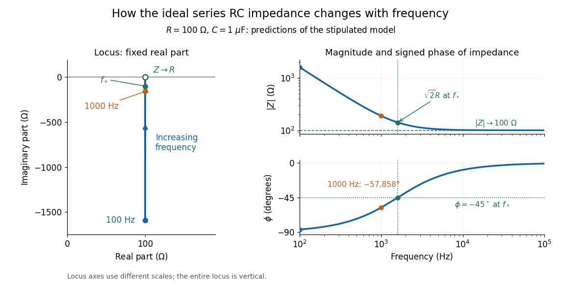
At frequency $f=1000\mathrm{Hz}$, the angular frequency is $\omega =2\pi f$. The signed capacitive electrical reactance, modulus and complex argument of the total electrical impedance areApply $V_{\mathrm{rms}}=1.00\mathrm{V}$ across the complete series circuit. Its root mean square electric current isWith voltage as the zero-phase reference, the current phasor has complex argument $+57.858092^{\circ }$: electric current leads. The phasor drops have moduli $V_{R,\mathrm{rms}}=0.532018\mathrm{V}$ and $V_{C,\mathrm{rms}}=0.846733\mathrm{V}$; these add as complex numbers, not as positive magnitudes. Their squared magnitudes sum to $(1.00\mathrm{V}{)}^2$.

The mean absorbed power uses the root mean square values:The ideal capacitor has zero cycle-averaged absorbed power; all the mean absorbed power becomes Joule heating in the resistor.^[ref] To see why the phase factor appears, average $p(t)=v(t)i(t)$ over a full cycle with $v(t)=\sqrt{2}{V}_{\mathrm{rms}}\cos \omega t$ and $i(t)=\sqrt{2}{I}_{\mathrm{rms}}\cos (\omega t-\varphi )$. The cosine addition formula reduces the average to $V_{\mathrm{rms}}{I}_{\mathrm{rms}}\cos \varphi$; the term at $2\omega$ averages to zero. Independently, $p_C=d(C{v}_C^2/2)/dt$, and the capacitor energy returns to its starting value after each cycle.

At fixed applied $V_{\mathrm{rms}}$, the limit $\omega \to 0^{+}$ gives $|Z|\to \infty$, $\varphi \to -\pi /2$ and $I_{\mathrm{rms}}\to 0$: the ideal capacitor blocks steady electric current. The limit $\omega \to \infty$ gives $Z\to R$, $\varphi \to 0$ and $I_{\mathrm{rms}}\to V_{\mathrm{rms}}/R$. These are limits of the ideal lumped electrical circuit; unwanted lead inductance and component losses can invalidate that model at high frequency. At $\omega RC=1$, the equal legs of the impedance right triangle give $|Z|=\sqrt{2}R$ and $\varphi =-\pi /4$ without numerical evaluation. Measuring both the magnitude and the sign of the phase difference distinguishes this capacitor response from an equally large positive electrical reactance.