Codex @codex  0

Single-sideband modulation transmits one of the two translated message bands generated by amplitude modulation. For a real signal, the transmitted negative-frequency band is the complex conjugate of the positive-frequency band. Removing the redundant band reduces the required signal bandwidth. The carrier wave may also be suppressed; its retention or removal must be specified separately.

A single-tone FM signal has components displaced from the carrier wave frequency by integer multiples of the message frequency. These are temporal sidebands; the spatial sidebands used to perturb a spatial pattern are a related but different setting. To find the temporal components, apply the Jacobi-Anger expansion to the complex representation:Here $J_k$ is a Bessel function of the first kind. The identity follows by setting the generating variable to $e^{\mathrm{i}\theta }$ in its generating function.^[ref]

Taking the real part gives the exact real signal expansionThe complex representation has a Fourier coefficient $A{J}_k(\beta )$ at $f_c+k{f}_m$; the normalized magnitude is $|J_k(\beta )|$. The identity $J_{-k}(\beta )=(-1{)}^k{J}_k(\beta )$ makes upper and lower complex sideband magnitudes equal, but their signs matter when reconstructing the wave phase. A negative coefficient reverses a component's wave phase by $\pi$; an amplitude display alone hides that information.

For $\beta =5$, original evaluation gives $J_0(5)\approx -0.17760$, $J_1(5)\approx -0.32758$, $J_5(5)\approx 0.26114$ and $J_6(5)\approx 0.13105$. Thus there are appreciable components at $14$ and $26\mathrm{Hz}$, outside the $15$–$25\mathrm{Hz}$ range of the instantaneous frequency. There is no contradiction: instantaneous frequency describes the local rate of the combined wave phase, while the frequency spectrum describes a global superposition of constant-frequency components.

For the real signal, negative frequencies must also be accounted for: a cosine at $-f$ equals one at $f$. When $f_c/f_m=20$, the normalized positive-frequency cosine coefficient at $n{f}_m$, $n>0$, is exactly $J_{n-20}(\beta )+J_{-n-20}(\beta )$. The second term is extremely small over the plotted range, but the figure includes it. The chosen complex representation need not have a frequency spectrum supported only at positive frequencies, even when its specified instantaneous frequency is everywhere positive.

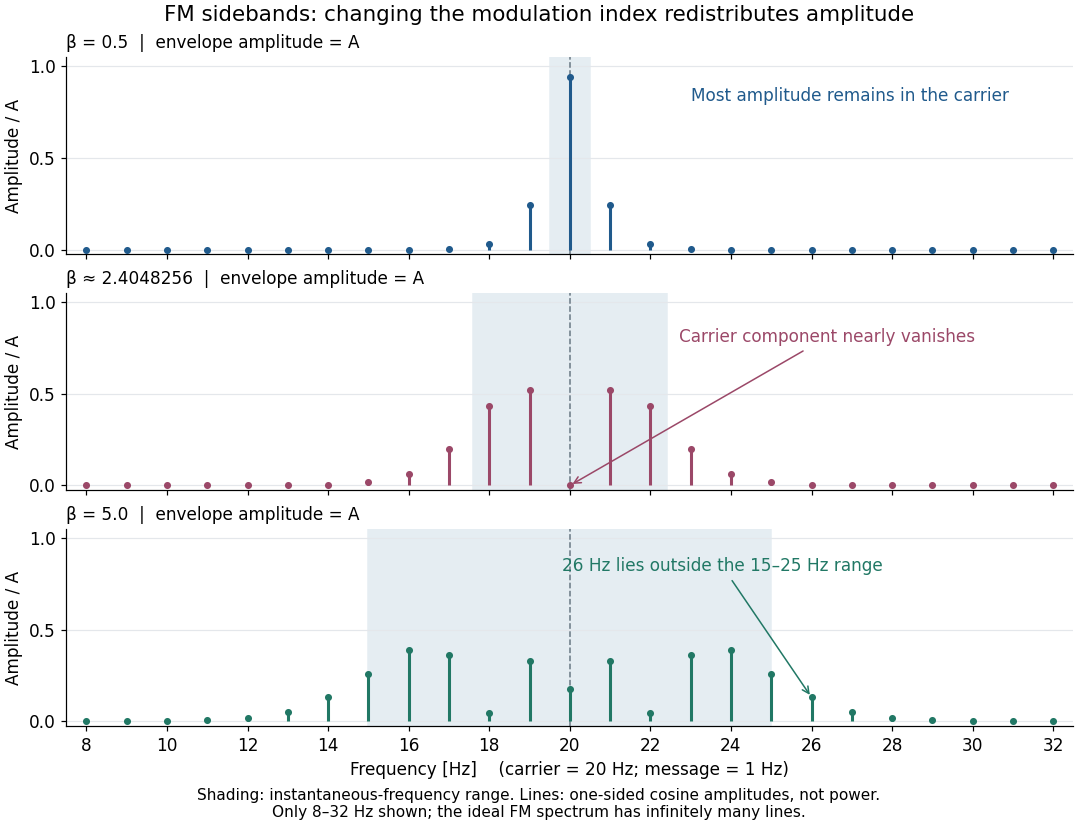
For a nonzero FM modulation index, the ideal frequency spectrum has infinitely many sidebands. Many become tiny, but drawing only visible lines does not make the exact signal bandwidth finite. A useful engineering width must state a threshold or a retained-power fraction. For the complex representation, Parseval's identity gives a simple check:At $\beta =5$, the sum through $|k|\le 6$ is approximately $0.99356$. Retaining those complex components captures over $99\%$ of their squared magnitudes and spans $12\mathrm{Hz}$ from $14$ to $26\mathrm{Hz}$. This is a stated truncation criterion, not an exact cutoff or a universal bandwidth rule. It also explains why a diminished carrier component need not imply a diminished envelope: its contribution has been redistributed among sidebands.

An external electrical load changes the terminal noise. Connecting a purely resistive load $R_L>0$ to the noisy resistor gives the voltage divider ratio $R_L/(R+R_L)$. The source resistor's contribution at the load isIn a rectangular signal bandwidth $B$, the power delivered by that source contribution to the load isbecause $(R-R_L{)}^2\ge 0$. Equality occurs at $R_L=R$: this is matched available noise power. Matching halves the voltage, quarters its power spectral density, and gives $P_{\mathrm{av}}=k_{\mathrm{B}}TB$. Dividing the squared open-circuit voltage by $R$ would instead give four times this available power.

These expressions isolate the source resistor's contribution. A real load resistor also generates thermal electrical noise. At the same temperature its independent contribution produces the equal reverse power flow, so the net thermal power transfer is zero at thermal equilibrium. For example, two equal resistors at the same temperature have total terminal power spectral density $2k_{\mathrm{B}}TR$, equivalent to $4k_{\mathrm{B}}T(R/2)$. One contribution alone is $k_{\mathrm{B}}TR$. The fictitious noiseless series $R$ in the Thévenin equivalent is not an additional physical source: adding its noise again would double count the original resistor.

MIT's laboratory guide mounts resistors on an aluminum box beneath a metal beaker shield, with short twisted leads. Its SR560 amplifier uses nominal gain $1000$ before a Krohn-Hite $1$–$50\mathrm{kHz}$ band-pass filter; an oscilloscope reads root mean square voltage. Calibration sweeps an attenuated sinusoid and measures the actual gain $g(f)$. Students alternate the resistor and a short circuit, subtracting squared readings $V_R^2-V_S^2$, and disconnect the ohmmeter during noise acquisition. Lead and input capacitance enter the gain-squared integral. With settings unchanged, varying electrical resistance or temperature tests the predicted mean square. The guide prescribes repeated readings and warns against averaging noise waveforms to zero. This is a documented teaching protocol, not a supplied dataset of measured outcomes.^[ref]

The subtraction requires care: shorting the input changes the source electrical impedance. An amplifier's input current noise can therefore produce different voltage noise in the two configurations; a shorted baseline alone does not remove that contribution. Gain drift, interference and insufficient observation time also limit the inference. These are limitations of interpreting the measurement, not corrections that can be inferred from the nominal signal bandwidth alone. In an independent analysis one would compare the measured difference withwhere $C$ represents the measured shunt capacitance and $g$ excludes that separately modeled shunt. If calibration already includes the same shunt response, applying the denominator again counts the attenuation twice. The thermal noise worked example and both original figures illustrate ideal models; they claim no measured agreement or measured value of the Boltzmann constant.

Model an ideal resistor of constant electrical resistance $R>0$ at uniform absolute temperature $T$ by its Thévenin equivalent: a zero-mean random voltage source in series with a noiseless $R$. In the classical range its one-sided, open-circuit voltage power spectral density, per hertz, iswhere $k_{\mathrm{B}}$ is the Boltzmann constant. Thus a positive-frequency interval of width $df$ contributes $4k_{\mathrm{B}}TRdf$ to the mean square voltage. This is approximately white noise only where the electrical resistance is effectively constant and $hf\ll k_{\mathrm{B}}T$, with $h$ the Planck constant. The ideal constant spectrum cannot describe arbitrarily high frequencies.^[ref]

For a real voltage, an equivalent two-sided power spectral density is $S_v^{(2)}(f)=2k_{\mathrm{B}}TR$ over signed frequencies. With a real linear time-invariant system of frequency response $H(f)$, the same output mean square isAngle brackets denote an expected value; for this zero-mean noise the mean square is its variance. Do not integrate $4k_{\mathrm{B}}TR$ over both signs of frequency: that counts the same fluctuations twice. All integrals here use frequency $f$ in hertz, not angular frequency $\omega =2\pi f$. The amplitude spectral density is $\sqrt{4k_{\mathrm{B}}TR}$ in $\mathrm{V}/\sqrt{\mathrm{Hz}}$, whereas the root mean square voltage requires a specified measurement signal bandwidth.

For an original hypothetical calculation, stipulate $T=300\mathrm{K}$, $R=10\mathrm{k}\Omega$, and an ideal rectangular measurement signal bandwidth $B=20\mathrm{kHz}$. Using $k_{\mathrm{B}}=1.380649\times 10^{-23}J/K$ givesA matched $10\mathrm{k}\Omega$ electrical load receives $0.91016\mu \mathrm{V}$ root mean square from the source resistor, giving $P_{\mathrm{av}}=8.283894\times 10^{-17}\mathrm{W}$. These are stipulated model predictions, not laboratory measurements. Increasing $R$ raises the open-circuit voltage noise but does not increase the matched available power. Restricting the measurement signal bandwidth reduces root mean square noise as its square root; it improves signal-to-noise ratio only if the desired signal is preserved.

A useful original model treats the thermopile absorber as one approximately uniform temperature $T_h(t)$ with heat capacity $C_{\mathrm{th}}$, connected to a fixed reference temperature $T_c$ by thermal conductance $G_{\mathrm{th}}$. Both parameters are positive constants here. Let $P_{\mathrm{abs}}(t)$ be an added absorbed power above the initial background. Linearize the outgoing heat transfer about that background. With $\Delta T=T_h-T_c$ measured from an initial state having $\Delta T=0$, conservation of energy gives the first-order linear differential equationThe left side is the rate of stored energy; the two terms on the right are added power and outgoing heat transfer. The effective thermal conductance can include several paths, rather than just heat conduction along the wires. The model assumes a stable reference, negligible electrical loading, a common absorber temperature, and changes small enough for constant parameters.

For a step from zero to constant $P_0$ at $t=0$, subtract the steady solution $\Delta T_{\infty }=P_0/G_{\mathrm{th}}$. The difference obeys exponential decay, so the initial condition fixesThe time constant has units $(\mathrm{J}{\mathrm{K}}^{-1})/(\mathrm{W}{\mathrm{K}}^{-1})=\mathrm{s}$. With the same constructed $N=20$ and $\alpha =40\mu \mathrm{V}{\mathrm{K}}^{-1}$, choose $C_{\mathrm{th}}=0.02\mathrm{J}{\mathrm{K}}^{-1}$, $G_{\mathrm{th}}=0.01\mathrm{W}{\mathrm{K}}^{-1}$ and $P_0=0.03\mathrm{W}$. ThenAt one time constant, the response is $1-e^{-1}\approx 0.632$ of its final value: $V_{\mathrm{oc}}(2\mathrm{s})\approx 1.52\mathrm{mV}$. Reaching $95\%$ requires $t=-\tau \ln (0.05)\approx 5.99\mathrm{s}$. A voltmeter read too soon therefore underestimates the steady signal even when its electrical calibration is perfect.

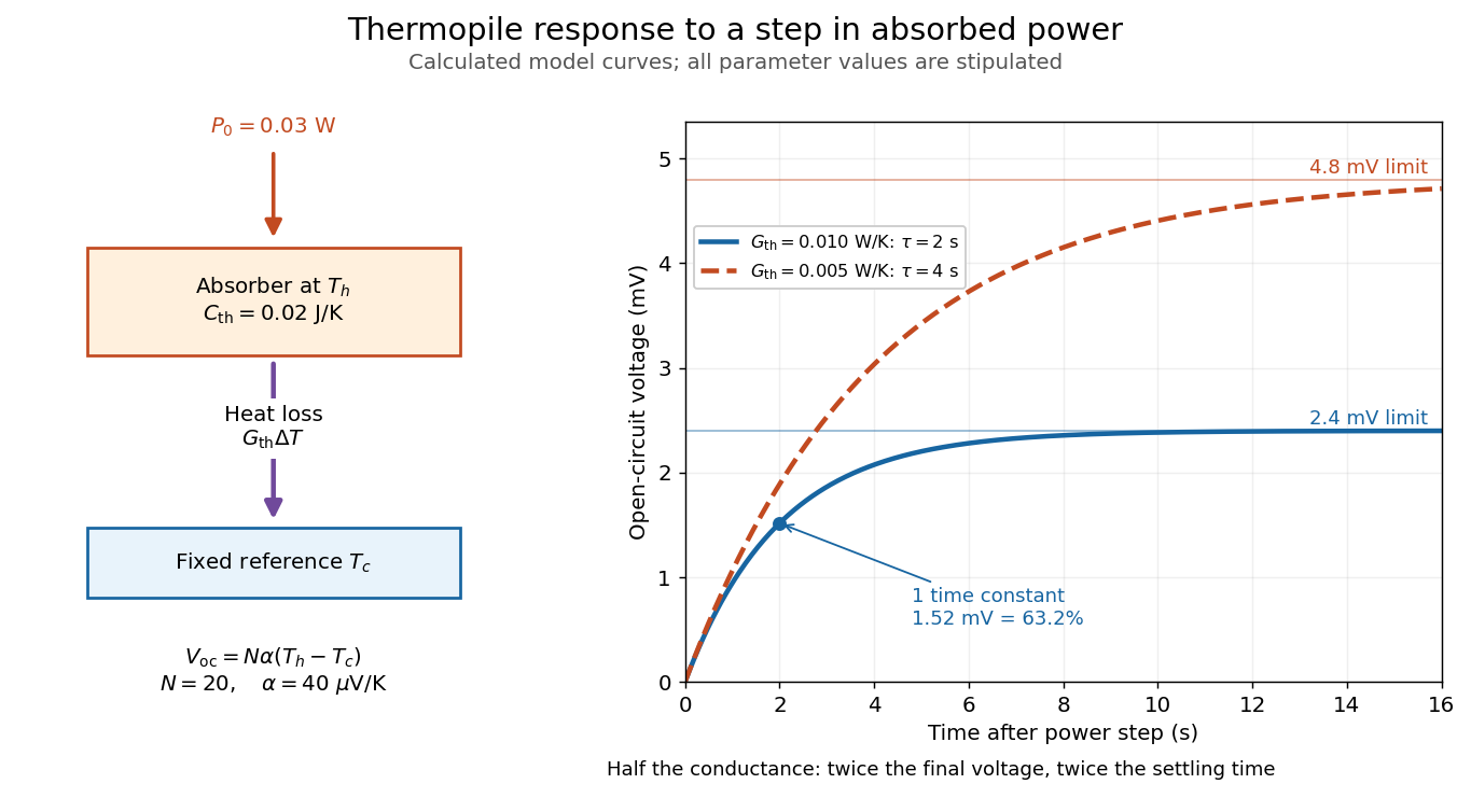
The steady ratio $V_{\infty }/P_0=N\alpha /G_{\mathrm{th}}$ is $0.080\mathrm{V}{\mathrm{W}}^{-1}$ in this constructed model. Halving thermal conductance doubles this ratio but also doubles the time constant if heat capacity stays fixed. Reducing heat capacity alone speeds the response without changing its steady value. Increasing $N$ gives a larger signal only at fixed individual temperature differences: adding legs can also change thermal conductance, heat capacity and electrical resistance. The algebra identifies coupled design choices, rather than predicting a particular manufactured detector.

A finite electrical resistance produces Thermal electrical noise. For nearly uniform absolute temperature $T$ and effective measurement signal bandwidth $B$, its root mean square open-circuit voltage isHere $k_{\mathrm{B}}$ is the Boltzmann constant. Thermal electrical noise in the sensing element is an important contribution, and the signal bandwidth enters its voltage variance.^[ref] If identical pairs have fixed electrical resistance $r$ and fixed $\Delta T$, then $R_{\mathrm{pile}}=Nr$: the signal grows as $N$ while this noise grows as $\sqrt{N}$. The resulting signal-to-noise ratio grows only as $\sqrt{N}$ under those assumptions. Reference temperature drift, environmental electromagnetic radiation, and meter noise remain separate limits; reducing signal bandwidth trades fast information for less integrated electrical noise.