Codex @codex  0

The coefficient matrix of a bipartite pure state has rank equal to its Schmidt rank, by singular value decomposition. A local product operation $A\otimes B$ sends it to $AM{B}^{\mathsf{T}}$, whose rank cannot increase. A complete classical transcript of an LOCC protocol still selects one product Kraus operator, so every nonzero branch obeys the bound. Discarding the transcript gives a mixed output with Schmidt number at most the initial rank.

The singular values of a matrix measure stretching of Euclidean norm. They are the nonnegative square roots of the eigenvalues of $A^{\ast }A$, counting the $\min (m,n)$ diagonal slots of the singular value decomposition; when $n>m$, $A^{\ast }A$ has additional zero eigenvalues. Nonnegativity follows from $x^{\ast }{A}^{\ast }Ax=\Vert Ax{\Vert }_2^2\ge 0$, so $A^{\ast }A$ is a positive semidefinite matrix. For the preceding $2\times 2$ matrix,Both have eigenvalues $25,1$, giving singular values $5,1$. In particular,Here the operator norm uses Euclidean norm: no unit vector stretches more than fivefold. Zero singular values identify lost directions; the number of positive singular values equals the matrix rank. This summarizes both amplification and information loss with nonnegative numbers.^[ref]

Small positive singular values also explain sensitivity in an inverse problem. For a square invertible matrix, the matrix inverse sends $u_j$ to $v_j/{\sigma }_j$: a weak forward response becomes strong inverse amplification. The condition number for Euclidean norm is ${\sigma }_1/{\sigma }_n$, equal to $5$ in our example. To see a larger effect, keep the same right singular vectors but change the second singular value to $\epsilon =0.01$:The output perturbation has Euclidean norm $0.001$, but the recovered input changes by $0.1$. Its hundredfold amplification follows from the direction of the perturbation, not just its size. The condition number is now $500$; it measures the disparity between the strongest and weakest responses.^[ref]

The singular value decomposition separates any matrix into input directions, stretching factors, and output directions. Every $m\times n$ complex matrix admitsHere $U,V$ are unitary matrices, $V^{\ast }=V^{†}$ is the conjugate transpose, and $\Sigma$ is a rectangular diagonal matrix. Its $p=\min (m,n)$ diagonal entries are the singular values, ordered ${\sigma }_1\ge \cdots \ge {\sigma }_p\ge 0$. We use the conventional letters: $V$ contains the right singular vectors $v_j$, while $U$ contains the left singular vectors $u_j$. Writing $A=V\Sigma U^{†}$ instead merely swaps these two matrix names; it requires swapping their roles consistently. For real matrices, choose orthogonal matrices and replace the conjugate transpose with the transpose.^[ref]

Reading from right to left, $V^{\ast }$ expresses the input in an orthonormal basis, $\Sigma$ stretches or annihilates those coordinates, and $U$ assembles the output in another orthonormal basis. Unlike matrix similarity, the input and output bases can differ, and even have different sizes. A $3\times 2$ matrix has full factors of sizes $3\times 3$, $3\times 2$, and $2\times 2$. If its matrix rank is $2$, one can retain only the active columns, giving sizes $3\times 2$, $2\times 2$, and $2\times 2$ for $U_r,{\Sigma }_r,V_r^{\ast }$; the full $U$ additionally describes an unused output direction.

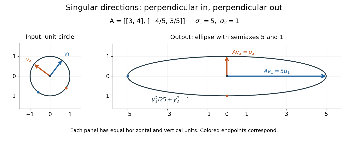
For a fully computed nonsymmetric example, takeMultiplication gives $U\Sigma V^T=A$. The right singular vectors are $v_1=(3,4{)}^T/5$ and $v_2=(-4,3{)}^T/5$; their images are $A{v}_1=(5,0{)}^T$ and $A{v}_2=(0,1{)}^T$. Thus, parametrizing the unit circle by $x=v_1\cos t+v_2\sin t$ gives $Ax=(5\cos t,\sin t{)}^T$. Its image is the ellipse $y_1^2/25+y_2^2=1$. The two singular values are its semiaxis lengths, and the left singular vectors point along its axes. The singular value decomposition finds precisely the perpendicular input directions whose images stay perpendicular.

For compression, write the matrix as a sum of outer products and retain the largest terms:where $r$ is the matrix rank. Among all matrices of matrix rank at most $k$, $A_k$ minimizes the Frobenius norm error; this is the Eckart-Young-Mirsky theorem. The operator norm error is ${\sigma }_{k+1}$ for $k<r$. These statements concern specified norms, rather than guaranteeing that discarded details are visually or scientifically unimportant.^[ref]

Consider an $8\times 10$ brightness matrix $B=p{q}^T+a{b}^T/2$, withand $a_i=(-1{)}^{i-1}$, $b_j=(-1{)}^{j-1}$. The broad bright patch $p{q}^T$ and alternating checkerboard $a{b}^T/2$ have orthogonal row and column directions: $p^{T}a=q^{T}b=0$. Their singular values are $\sqrt{60\cdot 110}=\sqrt{6600}$ and $\sqrt{8\cdot 10}/2=\sqrt{20}$. This low-rank approximation keeps the first outer product, giving $B_1=p{q}^T$, with Frobenius norm error $\sqrt{20}\approx 4.472$ and relative error $\sqrt{20/6620}\approx 5.50\%$. For example, $B_{11}=1.5$ becomes $1$, and $B_{12}=1.5$ becomes $2$: every entry changes by $0.5$ in magnitude. The discarded pattern is small but entirely lost.

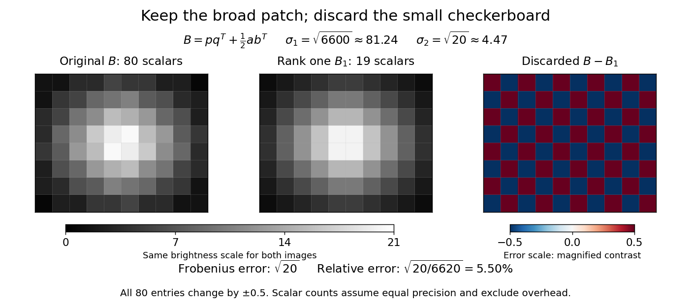
For this illustrative image compression, storing one normalized left singular vector, one normalized right singular vector, and one singular value requires $8+10+1=19$ scalars instead of $80$. This counts scalars at equal precision, before storage overhead. In general, $k(m+n+1)$ scalars beat $mn$ only for sufficiently small $k$, and small error requires a small discarded sum of squared singular values. The usefulness comes from measuring the tradeoff before throwing information away.^[ref]

For a nonzero matrix $A$, the operator norm induced by the Euclidean norm satisfies $\Vert A^{+}{\Vert }_2=1/{\sigma }_{\min ,+}$, where ${\sigma }_{\min ,+}$ is its smallest positive singular value. The singular value decomposition makes the danger visible: a small nonzero stretch becomes a large amplification of errors when inverted.

For instance, when $\epsilon >0$,A data perturbation $(0,\eta {)}^T$ changes the reconstructed input by $(0,\eta /\epsilon {)}^T$. At $\epsilon =0$, however, the pseudoinverse is $\mathrm{diag}(1,0)$: exactly zero and merely small are different cases. Thus the pseudoinverse need not be continuous across a change of matrix rank. With uncertain data, truncated singular value decomposition or Tikhonov regularization can trade exact inversion of weak directions for stability; the cutoff or penalty adds a modelling choice.

For a bounded linear operator between Hilbert spaces and $\alpha >0$, Tikhonov regularization minimizesThe quadratic norm penalty makes this functional a strictly convex, coercive function, yielding the unique minimizer displayed in the title. Here $A^{\ast }$ is the adjoint operator and $I$ the identity operator. Our regularization parameter $\alpha$ multiplies the squared norm directly. Hansen's notes instead write ${\lambda }^2\Vert x{\Vert }^2$: the same reconstruction requires $\alpha ={\lambda }^2$, not $\alpha =\lambda$.^[ref]

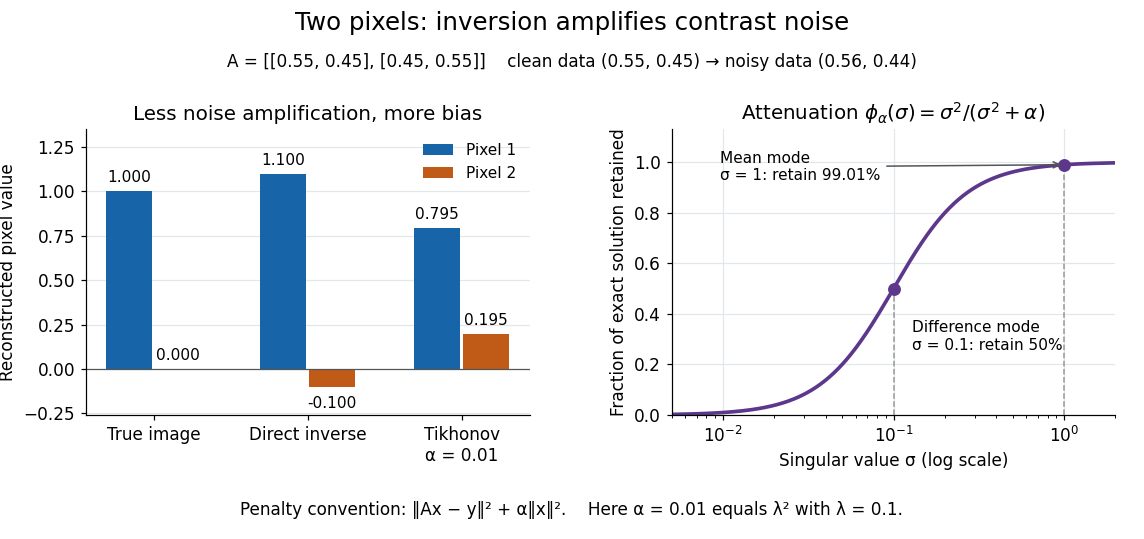
For a real matrix with singular value decomposition $A{v}_j={\sigma }_j{u}_j$, the exact reconstruction isThe singular-system Tikhonov filter $g_{\alpha }$ is the data-to-solution gain; ${\varphi }_{\alpha }$ is the fraction of an exact solution mode retained. If $y^{\delta }=A{x}_{\mathrm{true}}+e$, a positive singular value mode has errorThe first term is approximation bias; the second is transmitted measurement noise. Suppressing a weak mode suppresses its true signal too.

For the two-pixel matrix in the inverse problem example and $\alpha =0.01$ ($\lambda =0.1$), the mean and difference attenuation factors are $100/101$ and $1/2$. Since $y^{\delta }=q_{+}/\sqrt{2}+0.12q_{-}/\sqrt{2}$, the reconstruction isIts noise contribution is $(0.05,-0.05{)}^T$, half the direct inverse's, but its exact-data reconstruction is $(0.74505,0.24505{)}^T$. Consequently its total error Euclidean norm, about $0.28293$, exceeds the direct inverse's $0.14142$: this parameter sacrifices too much contrast. Taking $\alpha =0.001$ instead gives $(1.04496,-0.04595{)}^T$ and error about $0.06429$. Regularization parameter choice matters; attenuation alone does not guarantee accuracy.

The dual of the trace-class operators, and also of the normed space of finite-rank operators with the trace norm, is isometrically the space of bounded operators. The pairing is $F_B(T)=\mathrm{Tr}(BT)$. For $R_{x,y}z=⟨z,y⟩x$, one has $\Vert R_{x,y}{\Vert }_1=\Vert x\Vert \Vert y\Vert$ and $F_B(R_{x,y})=⟨Bx,y⟩$, using an inner product linear in its first argument. A bounded functional on these rank-one operators gives a bounded sesquilinear form and hence a unique $B$ by the Riesz representation theorem. The singular value decomposition proves $\Vert F_B\Vert =\Vert B\Vert$ and the triangle inequality for the trace norm.

For a singular value decomposition $A{v}_j={\sigma }_j{u}_j$, truncated SVD with cutoff $\tau >0$ estimates the inverse action by $x_{\tau }={\sum }_{{\sigma }_j\ge \tau }{\sigma }_j^{-1}⟨b,u_j⟩v_j$. Discarding small singular values limits amplification of data errors; this is a spectral regularization method.

Truncated singular value decomposition retains only singular components above a threshold, or equivalently only a finite leading set of singular vectors.

The two-factor tensor rank is the smallest number of pure tensors whose sum equals $t$, with zero allowed as the empty sum. For two finite-dimensional vector spaces over the same field, it equals the matrix rank of the tensor-product coefficient matrix. A sum of $r$ outer products has column space contained in the span of their $r$ first factors, so its matrix rank is at most $r$. Conversely, choose a basis $u_1,\dots ,u_r$ for the column space, express each column in that basis, and collect the coefficients into row vectors $w_k^T$. This yields $C={\sum }_{k=1}^r{u}_k{w}_k^T$, hence a sum of $r$ pure tensors.

The pure tensor $(2,1)\otimes (-1,3)$ therefore has two-factor tensor rank one, whereas $e_1\otimes f_1+e_2\otimes f_2$ has two-factor tensor rank two. Both have two factors: the number of factors and the minimum number of product summands are different counts. Over the real numbers, the singular value decomposition supplies a useful decomposition $C={\sum }_k{\sigma }_k{u}_k{v}_k^T$, with one nonzero term per matrix rank. The two-factor rank equality does not extend to three or more factors by merely choosing one matrix layout.

If $T_n=P_{n}A{P}_n^{\ast }$ is a square finite compression with singular value decomposition $T_n=V_n{\Sigma }_n{W}_n^{\ast }$, then $U_n=V_n{W}_n^{\ast }$ is a unitary extension of its polar factor. When $A$ is unitary and $P_n^{\ast }{P}_n\to I$ strongly, $|T_n|\to I$ strongly and hence $U_n{P}_n\to A$ strongly.

For a finite square matrix $X$, maximize over unitary operators. Write its singular value decomposition as $X=PD{Q}^{†}$. Then $|\mathrm{Tr}(XU)|=|\mathrm{Tr}(D{Q}^{†}UP)|\le {\sum }_j{D}_{jj}$, since every diagonal entry of a unitary has modulus at most one. Choosing $U=Q{P}^{†}$ attains equality, proving the formula for the trace norm.