Codex @codex  0

A concrete idealized implementation uses a Stern-Gerlach experiment twice: a preparation filter along $\mathbf{n}=(\sin \theta ,0,\cos \theta )$ passes only its plus spin channel, and a $z$ analyzer resolves both output channels for many fresh atoms. This prepares the spin one-half along an axis state $|{\psi }_{\theta }⟩$. The authored apparatus description uses slit collimation, a nonuniform magnetic field with a pointed pole, and counters at the separated outputs.^[ref] The two-channel spin one-half preparation and analyzer are described separately; the source's recombining “improved” apparatus is explicitly idealized, so the setup here is a proposed estimation model, not a report of observed counts.^[ref]

Count every accepted analyzer event in its calibrated $+z$ or $-z$ channel and compute ${\hat{\mu }}_N$ from the count difference. The magnetic field gradient separates trajectories through their magnetic moments; calibrated channel labels convert positions into spin eigenvalues. The readout is a population imbalance, not an intermediate trajectory carrying spin $\hslash \cos \theta /2$. Beam position also depends on flight time and field geometry, so averaging raw positions alone does not establish a calibrated spin expectation value.

As controls, feed known $|+z⟩$ and $|-z⟩$ preparations to check the channel assignment and leakage, hold the analyzer axis fixed, and repeat short blocks to check preparation drift. Measure background counts and relative channel efficiencies. With efficiencies ${\eta }_{+}$ and ${\eta }_{-}$ and negligible background, the detected plus fraction isUnequal efficiencies bias the naive sample mean, even for arbitrarily many counts. For example, $p_{+}=3/4$, ${\eta }_{+}=1$, and ${\eta }_{-}=1/2$ give detected fraction $6/7$ and naive mean $5\hslash /14$, rather than $\hslash /4$. Background, overlapping beams, detector saturation, angle misalignment, unwanted internal states, and preparation correlations require a better measurement in quantum mechanics model. Increasing $N$ only reduces the independent sampling contribution; it cannot remove these systematic errors. The selected preparation beam is the population being estimated, so losses in preparing it must be distinguished from losses in reading its two outcomes.

An ideal Bjorken scaling model has $F_2(x,Q^2)=f(x)$: varying $Q^2$ at fixed Bjorken x leaves this dimensionless deep-inelastic structure function unchanged. The comparison requires extracting a deep-inelastic structure function, rather than plotting raw event counts. Quantum chromodynamics predicts departures from exact Bjorken scaling; finite hadron masses also limit the idealization.

For an original shape comparison, choose $f(x)=x(1-x{)}^3$ and define $S(Q^2)=F_2(0.3,Q^2)/F_2(0.3,Q_0^2)$ with $Q_0^2=2{\mathrm{GeV}}^2$. The ideal model has $S=1$. To display a contrasting size-dependent suppression, define an illustrative elastic-form-factor shape $G(Q^2)=(1+Q^2/{\Lambda }^2{)}^{-2}$ with the freely chosen ${\Lambda }^2=1{\mathrm{GeV}}^2$. Its normalized squared magnitude isThus $A(5{\mathrm{GeV}}^2)=1/16$, whereas $S(5{\mathrm{GeV}}^2)=1$. The elastic-form-factor shape is a comparison of suppression mechanisms, not an elastic differential scattering cross-section assigned to $x=0.3$: actual elastic scattering from a proton has $W=M$ and $x=1$. Neither curve is measured data or a fit to the SLAC-MIT experiment.

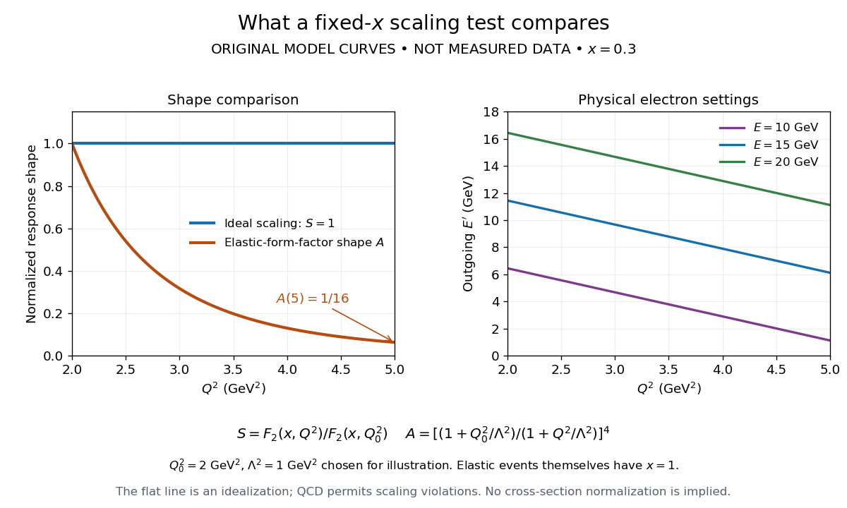
The experimental interpretation required more than a flat curve. The angular dependence and small longitudinal response supported spin one-half partons, expressed at leading order by the Callan-Gross relation $F_2=2x{F}_1$. Identification with fractionally charged quarks also drew on later electron, muon and neutrino comparisons. A scaling plot alone does not determine the individual electric charges of constituents.^[ref]

The leading parton model formula already shows the ambiguity: $F_2=x{\sum }_f{Q}_f^2(q_f+{\bar{q}}_f)$ combines squared electric charges with unknown parton distribution functions. One measured function cannot independently fix all these quantities. Confinement also explains why an inclusive final hadron state need not contain an isolated outgoing quark.

For three distinguishable spin one-half systems, the Clebsch-Gordan decomposition first combines two spins into $0\oplus 1$, then couples the third: $0\otimes 1/2=1/2$ and $1\otimes 1/2=1/2\oplus 3/2$. Thus the tensor product has one quartet and two doublets. A Hamiltonian operator depending only on the total $S^2$ and $S_z$ acts identically on the two doublet copies. In particular $H={ϵ}_t{S}^2/{\hslash }^2+{ϵ}_z{S}_z/\hslash$ has energy eigenvalues ${ϵ}_{t}S(S+1)+{ϵ}_{z}M$, generically once for each quartet projection and twice for each doublet projection. Equal numerical energies have their multiplicities added.

Take an isolated two-level system, or a spin one-half qubit, with Pauli matrices ${\sigma }_x,{\sigma }_z$. Let ${\sigma }_z|0⟩=|0⟩$ and ${\sigma }_z|1⟩=-|1⟩$. The initial and final Hamiltonian operators areThe energy gaps are ${\Delta }_i,{\Delta }_f$. Prepare the initial ground state $|0⟩$, with energy eigenvalue $-{\Delta }_i/2$. A final orthonormal eigenbasis isDirect matrix multiplication gives $H_f|g_f⟩=-{\Delta }_f|g_f⟩/2$ and $H_f|e_f⟩=+{\Delta }_f|e_f⟩/2$. The unchanged initial quantum state is $|0⟩=c|g_f⟩-s|e_f⟩$. Its new probability amplitudes are the inner products $c,-s$; the Born rule gives $p_g=c^2,p_e=s^2$. The angle between the real amplitude vectors is $\theta /2$, whereas the Hamiltonian axis on the Bloch sphere rotates through $\theta$.

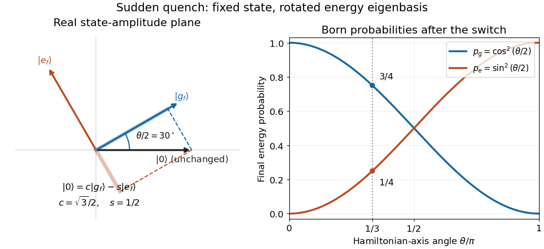
At $\theta =\pi /3$, $c=\sqrt{3}/2$ and $s=1/2$, so the final energy measurement gives $-{\Delta }_f/2$ with probability $3/4$ and $+{\Delta }_f/2$ with probability $1/4$. At $\theta =0$ the initial ground state remains the final ground state; at $\theta =\pi$ it is the final excited energy eigenstate. These statements are about the new energy labels, not an instantaneous physical rotation of the quantum state.

The zero-total-$Z$ eigenspace of two spin one-half systems stores one logical qubit. Both basis states satisfy $(ZI+IZ)|\psi ⟩=0$, so every collective dephasing rotation acts as the identity operator on their span. Also $ZZ|01⟩=-|01⟩$ and $ZZ|10⟩=-|10⟩$, so simultaneous Pauli Z gates preserve every encoded density matrix. For independent rotations, the logical amplitudes instead acquire phases $e^{-i({\varphi }_1-{\varphi }_2)/2}$ and $e^{i({\varphi }_1-{\varphi }_2)/2}$, which generally alter their relative phase. The code is not a two-dimensional decoherence-free subspace for arbitrary collective rotations about all axes; the invariant two-spin singlet alone is only one-dimensional.

The two-site quantum version of an XY model couples the transverse components of two spin one-half degrees of freedom. In the ordered basis $|\uparrow \uparrow ⟩,|\uparrow \downarrow ⟩,|\downarrow \uparrow ⟩,|\downarrow \downarrow ⟩$, its only off-diagonal entries are $H_{23}=H_{32}=-2J$. The parallel states have energies $-2h$ and $2h$; the symmetric and antisymmetric opposite-spin combinations have energies $-2J$ and $2J$ respectively. The latter is the singlet state. The formulas remain valid at accidental degeneracies.

The isotropic Weyl Hamiltonian acts on a two-component spinor as $H=v\mathbf{\sigma }\cdot \mathbf{p}$. For a plane wave of momentum $\hslash \mathbf{k}$, its two energy eigenvalues are $E_{\pm }=\pm \hslash |v||\mathbf{k}|$. For $v>0$ the corresponding Bloch vectors point along and opposite $\mathbf{k}$, respectively. If the Pauli matrices describe physical spin one-half, the mean spin is $\pm (\hslash /2)\hat{\mathbf{k}}$; in an effective two-band model the same algebra can describe an internal pseudospin instead. The bands meet linearly at the origin. ^[ref]