Two-level sudden quench ($p_g={\cos }^2(\theta /2),p_e={\sin }^2(\theta /2)$)

Take an isolated two-level system, or a spin one-half qubit, with Pauli matrices ${\sigma }_x,{\sigma }_z$. Let ${\sigma }_z|0⟩=|0⟩$ and ${\sigma }_z|1⟩=-|1⟩$. The initial and final Hamiltonian operators areThe energy gaps are ${\Delta }_i,{\Delta }_f$. Prepare the initial ground state $|0⟩$, with energy eigenvalue $-{\Delta }_i/2$. A final orthonormal eigenbasis isDirect matrix multiplication gives $H_f|g_f⟩=-{\Delta }_f|g_f⟩/2$ and $H_f|e_f⟩=+{\Delta }_f|e_f⟩/2$. The unchanged initial quantum state is $|0⟩=c|g_f⟩-s|e_f⟩$. Its new probability amplitudes are the inner products $c,-s$; the Born rule gives $p_g=c^2,p_e=s^2$. The angle between the real amplitude vectors is $\theta /2$, whereas the Hamiltonian axis on the Bloch sphere rotates through $\theta$.

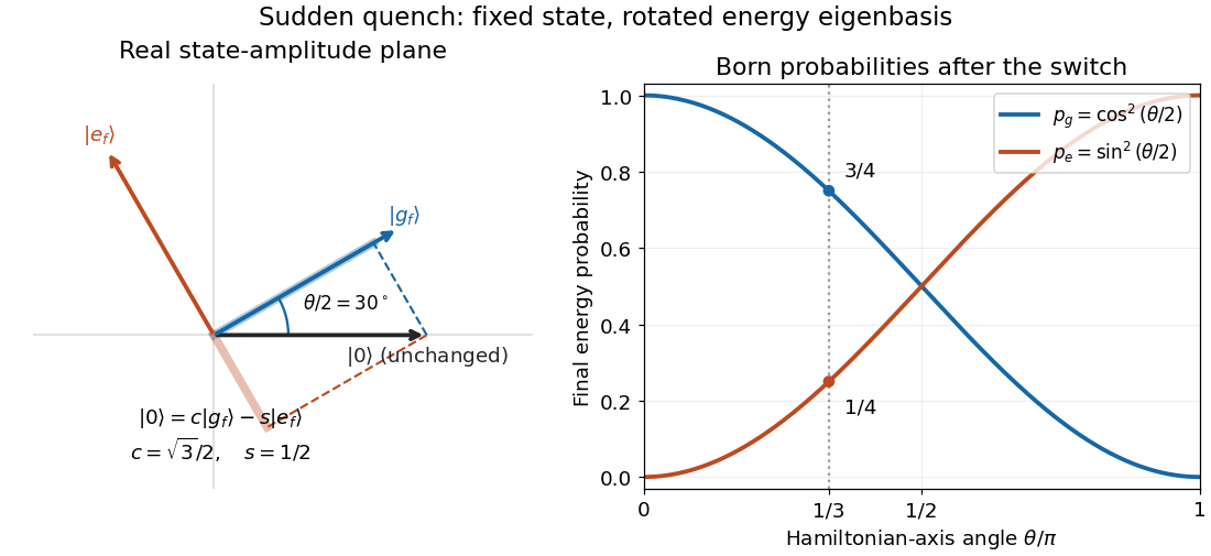
At $\theta =\pi /3$, $c=\sqrt{3}/2$ and $s=1/2$, so the final energy measurement gives $-{\Delta }_f/2$ with probability $3/4$ and $+{\Delta }_f/2$ with probability $1/4$. At $\theta =0$ the initial ground state remains the final ground state; at $\theta =\pi$ it is the final excited energy eigenstate. These statements are about the new energy labels, not an instantaneous physical rotation of the quantum state.

The drive can supply or extract work while the quantum state stays approximately fixed. For a differentiable bounded Hamiltonian operator, the Schrödinger equation givesThe state-evolution terms cancel, leaving the external drive's power. For a finite ideal step the change in mean energy is $⟨\psi |H_f-H_i|\psi ⟩$. Thus conservation of energy for a closed system with a time-independent Hamiltonian operator does not assert conservation of the driven subsystem's energy during switching.

Specify work operationally by two energy measurements: one before the switch and one after. For the prepared initial ground state, the first outcome is definite; the second samples the new Born rule probabilities. This protocol gives a distribution of measured energy differences, rather than generally the measurement distribution of the single operator $H_f-H_i$.^[ref]and henceFor ${\Delta }_i={\Delta }_f=\Delta$ and $\theta =\pi /3$, the work is $0$ or $\Delta$, with probabilities $3/4$ and $1/4$; its expectation is $\Delta /4$ and its variance is $3{\Delta }^2/16$. The initial mean energy $-\Delta /2$ becomes $-\Delta /4$. Using different initial and final scalar offsets would also shift the measured work; the displayed Hamiltonian operators fix that convention explicitly.

After the quantum quench, hold $H_f$ fixed and evolve without an intervening energy measurement. The unitary time evolution isProjection onto the original $|0⟩$ gives probability amplitude $c^2{e}^{+i{\Delta }_{f}t/(2\hslash )}+s^2{e}^{-i{\Delta }_{f}t/(2\hslash )}$. Squaring its modulus yields the two-level quantum return probabilityTheir sum is one. For $\theta =\pi /3$, the first minimum of $P_0$ is $1/4$ at $t=\pi \hslash /{\Delta }_f$, and the return is complete at $T=2\pi \hslash /{\Delta }_f$. At $\theta =0$ or $\pi$ there is no oscillation, because the initial quantum state is already a final energy eigenstate.

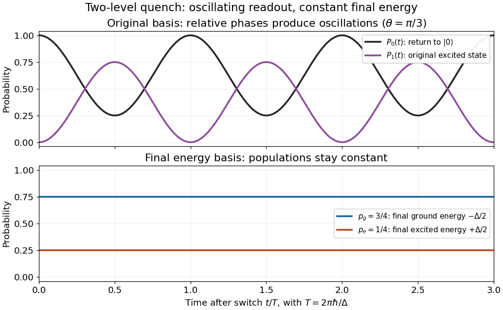
Changing measurement basis reveals the evolving relative quantum phase. Measuring the final energy first instead destroys this quantum coherence between final energy eigenstates in the unconditioned ensemble: its later original-basis return probability is $c^4+s^4=1-\frac{1}{2}{\sin }^2\theta$, equal to $5/8$ for this example. That constant differs from the oscillation of the unmeasured pure state. The work protocol and the oscillation protocol therefore use separate preparations.