Codex @codex  0

Let $q_0$ be the stationary point and let $H=D^2\beta (q_0)$ be its real symmetric Hessian matrix. First suppose the stationary point is interior and nondegenerate, the oscillatory integral amplitude and oscillatory integral phase are sufficiently smooth, and boundary contributions are absent or smaller than the stationary contribution. Diagonalize $H$ by an orthogonal change of coordinates, with eigenvalues $h_1,h_2$. Locally,Scaling each principal coordinate by ${\lambda }^{-1/2}$ and evaluating its Fresnel integral gives the two-dimensional stationary-phase formula:Here $\mathrm{sgn}H$ is the number of positive eigenvalues minus the number of negative ones: $2$, $0$ or $-2$. The formula gives the leading nonzero term when $\alpha (q_0)\ne 0$. A partition of unity isolates this neighbourhood; integration by parts away from stationary points makes the remaining interior contribution smaller. For a smooth compactly supported oscillatory integral amplitude the local error is $O({\lambda }^{-2})$.

The printed assumption of a single stationary point alone is insufficient for an unconditional answer. A degenerate oscillatory integral phase $\beta =x^4+y^2$ with a smooth oscillatory integral amplitude supported near the origin has only one stationary point, but scales as ${\lambda }^{-3/4}$. Boundary terms can also contribute at order ${\lambda }^{-1}$: on the unit disk with oscillatory integral amplitude one and $\beta =x^2+y^2$,whose stationary contribution is $i\pi /\lambda$ and whose boundary contribution is $-i\pi e^{i\lambda }/\lambda$. Thus the boxed formula is the standard nondegenerate interior stationary contribution, with the stated hypotheses; the data as printed do not determine all possible leading behaviours.

The linear elastic wave equation is $\rho {\mathbf{u}}_{tt}=(\lambda +\mu )\nabla (\nabla \cdot \mathbf{u})+\mu \Delta \mathbf{u}$. For a shear-horizontal wave, take $\mathbf{u}=(0,v(x,z,t),0)$ with no $y$ dependence. Its divergence vanishes, andRigid fixed boundaries require $v=0$ at $z=0,h$. The modes are $v=A\sin (q_{n}z)\cos (kx-{\omega }_{n}t)$ with $q_n=n\pi /h$, $n=1,2,\dots$, andThere is no $n=0$ displacement mode with these clamped boundary conditions. For $k>0$, the phase velocity and group velocity areThe phase velocity decreases from infinity to $c_s$, while the group velocity increases from zero to $c_s$; their product is $c_s^2$.

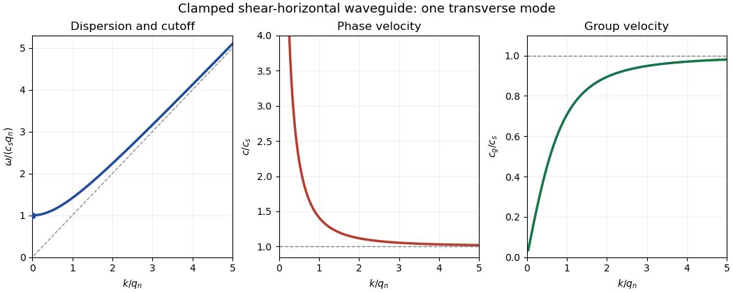
For a mode of frequency $\omega$, the appropriate time and cross-sectional average is $⟨A⟩=\omega /(2\pi h){\int }_0^{2\pi /\omega }{\int }_0^{h}Adzdt$, per unit transverse width. Its average kinetic energy density is $\rho A^2{\omega }^2/8$. The only nonzero strains are $e_{xy}=e_{yx}=v_x/2$ and $e_{yz}=e_{zy}=v_z/2$, while $e_{kk}=0$. Thus the elastic energy density is $\mu (v_x^2+v_z^2)/2$, whose average is $\mu A^2(k^2+q_n^2)/8$. The dispersion relation proves equality of average kinetic and elastic energies.

For the ray asymptotics of a clamped elastic waveguide mode, expand the localized initial displacement in transverse sine modes and Fourier transform in $x$. For a displacement released from rest, each mode evolves with $\cos ({\omega }_n(k)t)$. At $x=Vt$ the oscillatory phases are $t(kV\pm {\omega }_n(k))$. If $0<|V|<c_s$, one phase has a stationary point withThe stationary phase method gives a generic oscillatory amplitude proportional to $t^{-1/2}$ for each contributing mode. If the initial Fourier coefficient vanishes at the stationary point, that mode can decay faster; smooth localized data make the modal sum well behaved. If $|V|>c_s$, there is no stationary point. Repeated integration by parts gives rapid decay for smooth rapidly decaying data; for initially compactly supported displacement, finite propagation speed makes the displacement on that ray exactly zero after a sufficiently long time. These are the requested subsonic and super-shear-speed regimes.

Use inverse temperature ${\beta }_T=(k_{B}T{)}^{-1}$, reserving $\beta$ without a subscript for the critical exponent. Write $c=qJ$; each undirected bond occurs once, so the number of bonds is $Nq/2$. In the mean-field theory of the Ising model, write each Ising spin as ${\sigma }_i=m+\delta {\sigma }_i$ and neglect the product of fluctuations:The resulting independent-spin statistical Hamiltonian isThe constant corrects the double counting of interaction energy. The Ising spin sums now factorize and can all be evaluated:This is the approximate partition function at an assumed mean field; equilibrium fixes $m$ self-consistently. The corresponding Ising auxiliary mean-field free energy isIts equilibrium value gives the mean-field Helmholtz free energy in the imposed field. Away from a stationary point its parameter $m$ is an assumed field variable, not necessarily the actual mean Ising spin of that independent-spin distribution.

For the full small-$m$ expansion at fixed $h$, set $t_h=\tanh ({\beta }_{T}h)$ and $s_h={\mathrm{sech}}^2({\beta }_{T}h)$. Differentiating $\log \cosh z$ gives successive derivatives $t_h$, $s_h$, $-2t_h{s}_h$, and $2s_h(2-3s_h)$ at $z={\beta }_{T}h$. ThereforeAt zero field, spin inversion symmetry eliminates odd powers and this simplifies toThe quadratic coefficient changes sign and the quartic coefficient is positive atThus the zero-field mean-field prediction is a continuous, continuous phase transition: the stable zero spin magnetization develops two symmetry-related nonzero minima continuously below $T_c$.

Both requested routes give the same mean-field self-consistency equation. First, the one-spin expectation in the effective field isSecond, differentiating the Ising auxiliary mean-field free energy giveswhose stationary condition is precisely that mean-field self-consistency equation. Choose its stable, lowest-free-energy branch rather than every algebraic solution.

An equally useful mean-field approximation parametrizes the trial distribution by its actual mean Ising spin. Its probabilities are $(1\pm m)/2$, giving the Bragg-Williams free energy of the Ising modelThis energy-minus-entropy function has expansionIts stationary equation is $h=k_{B}T\mathrm{arctanh}m-cm$, again equivalent to the mean-field self-consistency equation. The two functions differ away from equilibrium, but agree on stationary branches: for $z={\beta }_T(h+cm)$ and $m=\tanh z$, the entropy bracket equals $mz-\log (2\cosh z)$. Their small-$m$ coefficients therefore need not agree at arbitrary temperature; at $T_c$ they have the same leading critical quartic coefficient $c/12$. This distinction prevents confusing the auxiliary-field expansion with the physical-magnetization variational expansion.

For the order-parameter critical exponent, expand the equation of state at $h=0$:On a nonzero stable branch,Hence $\beta =1/2$. The spontaneous magnetization is understood by selecting a branch with an infinitesimal field after the thermodynamic limit; a finite symmetric sample has zero exact zero-field mean Ising spin.

For the magnetic susceptibility per site, define $\chi =\partial m/\partial h$ with $h$ in energy units. Implicit differentiation givesAbove $T_c$, $m=0$ and $\chi =1/[k_B(T-T_c)]$. Below $T_c$, evaluated on a selected ordered branch, the expansion of $m^2$ gives $\chi \sim 1/[2k_B(T_c-T)]$. Thus the magnetic-susceptibility critical exponent is $\gamma =1$ on both sides, with different amplitudes. At $T=T_c$, the equation of state becomesso the critical-isotherm exponent is $\delta =3$. These are mean-field critical exponents, not a claim that neglecting fluctuations gives the exact Ising transition in every dimension.

Assume the scalar order parameter can take either sign. The cubic term breaks $m\mapsto -m$ symmetry, and a positive quartic coefficient bounds the Landau free energy below. Stationary points satisfyso, besides the disordered point $m=0$, the possible ordered points areThe disordered point has curvature $A^{\prime \prime }(0)=A_2$ and is locally stable when $A_2>0$. Nonzero stationary points first appear whenThat condition alone does not make them the equilibrium phase: one must compare their free energies.

At a nonzero stationary point, substitute $A_2=-A_{3}m-A_4{m}^2$ to obtainFor an ordered state to coexist with $A(0)=0$, this requiresBoth curvatures at phase coexistence are positive and equal to $2A_3^2/(9A_4)$. The barrier is at $m=-A_3/(3A_4)$. In fact the potential at phase coexistence factorizes:The two distinct minima are therefore explicit, with a finite jump in the order parameter whenever $A_3\ne 0$.

To state the equilibrium inequalities for either sign of $A_3$, put $m=-\mathrm{sgn}(A_3)\rho$ with $\rho \ge 0$. This sign always has lower energy than the opposite sign of equal magnitude. ThenThe bracket's minimum is $A_2/2-A_3^2/(9A_4)$. It follows thatThe favored ordered minimum, when it exists, isThus a first-order phase transition is possible and occurs when the coefficients cross the coexistence relation. There is no continuous transition between $m=0$ and the equilibrium ordered state while $A_3$ remains nonzero and $A_4$ remains finite and positive. The ordered state becomes globally favorable while $A_2$ is still positive, before the disordered curvature can vanish. Although a stationary solution tends to zero at $A_2=0$, it is not the global transition branch. A continuous transition would require eliminating the cubic term, outside the stated $A_3\ne 0$ condition.

The spinodal points clarify the metastable region: for $2A_3^2/(9A_4)<A_2<A_3^2/(4A_4)$ the ordered minimum is metastable; for $0<A_2<2A_3^2/(9A_4)$ the disordered minimum is metastable. At $A_2=0$ the disordered state loses local stability. These local-stability limits should not be mistaken for the first-order transition in a cubic-quartic Landau potential.

The first partial derivatives areBoth vanish at $(\lambda ,\lambda )$, so every positive diagonal point is a stationary point. The Hessian matrix there isIts eigenvectors $(1,1)$ and $(1,-1)$ have respective eigenvaluesThe zero eigenvalue reflects the entire line of nonisolated stationary points: $f(\lambda ,\lambda )=2$. In fact $f-2=(x-y{)}^2[1/(xy)-1/a^2]$, showing a non-strict local minimum when $\lambda <|a|$, a non-strict local maximum when $\lambda >|a|$, and values on both sides of two near $\lambda =|a|$. At that last point the whole Hessian matrix vanishes, so its signs alone cannot classify the point.

In the Landau theory approximation, choose the global minimum of the Landau free energy as a function of the magnetization. Since ${\mathcal{A}}_6>0$, the polynomial is a coercive function and a global minimum exists. The candidates are stationary points satisfyingCheck their values of the free-energy density; a stationary point or a metastable local minimum alone need not be the equilibrium state. Positive curvature ${\mathcal{A}}_2+3{\mathcal{A}}_4{m}^2+5{\mathcal{A}}_6{m}^4$ ensures local stability; when it vanishes, higher terms must be checked. The selected global minimum is the equilibrium magnetization within this approximation.

At zero magnetic field, equal opposite minima describe distinct phases exhibiting spontaneous symmetry breaking. A spontaneous magnetization is obtained by taking the thermodynamic limit before $h\to 0^{+}$ or $h\to 0^{-}$. A symmetric finite-volume average can instead have zero expectation even when the minima are nonzero. Thus one must specify the phase when interpreting the minimizer as the equilibrium expectation.

Discuss the zero-field phase boundaries, taking $h=0$ and writing $r={\mathcal{A}}_2$, $q={\mathcal{A}}_4$, $s={\mathcal{A}}_6>0$. This qualification matters because a conjugate field generally rounds the zero-field continuous transition. Nonzero stationary points satisfy $r+q{m}^2+s{m}^4=0$.

For $q>0$, the continuous phase transition occurs atOn the $r>0$ side the only stable phase is $m=0$; on the $r<0$ side the equilibrium global minima are $\pm m_0$ with $m_0^2\sim -r/q$. The magnetization therefore grows continuously from zero as $r$ changes sign.

For $q<0$, the first-order phase transition instead occurs while $r$ is positive. At phase coexistence, $m=0$ and $m=\pm m_0$ are equally deep global minimum points. With $a=m_0^2>0$, stationarity and equality of free energies giveEliminating $r$ gives $-q{a}^2/4-s{a}^3/3=0$, henceAt this coexistence value, the sextic even Landau potential factors as $f(m)=s{m}^2(m^2+3q/(4s){)}^2/6\ge 0$. This verifies that the three equal stationary values are global minima. Above this coexistence value of $r$ the disordered phase wins; below it the ordered phase wins, with a finite jump in the phase-selected magnetization. The values $r=0$ and $r=q^2/(4s)$ are the disordered and ordered spinodal points, respectively, not the coexistence boundary: the latter follows from the repeated root of $r+qa+s{a}^2=0$.

The two transition loci meet at the tricritical point,Two independent control parameters such as $T$ and $g$ can tune these two conditions. In a generic local phase diagram their coefficient map has a Jacobian matrix of rank two at the intersection; unspecified functions ${\mathcal{A}}_2(T,g)$ and ${\mathcal{A}}_4(T,g)$ do not by themselves determine the geometric orientation of the boundaries. The sextic term stabilizes this intersection and the negative-quartic first-order side.

For $0<V<\beta /(8{\ell }^2)$ there are two positive solutions $k_1\in (\ell ,\sqrt{3}\ell )$ and $k_2>\sqrt{3}\ell$, together with their negatives. The second derivative isEach negative stationary point has the conjugate contribution of its positive partner, because $A$ is real even and ${\Phi }_V$ is odd. ThereforeIf a leading amplitude vanishes, this gives a zero coefficient and a higher-order term supplies that branch's first nonzero contribution.

Use the real integral representation of the modified Bessel function of the second kindThe unique stationary point is the strict maximumThe Laplace approximation is consequentlyFor fixed $x>0$, as $\nu \to +\infty$,Substitution gives the required large-order asymptotic of the modified Bessel function of the second kind:

Introduce the orthogonal coordinatesThen the constraint and objective becomeThe Lagrange multiplier equations for a stationary point areIf $\lambda =0$, then $u=y=0$ and $v=\pm 1$, givingIf $\lambda \ne 0$, then $v=0$. The first two equations and the constraint implyConverting back to $(x,y,z)$ gives the other four points. Therefore all stationary points arewith matching signs, together withThe middle pair has $\varphi =1/2$, the last pair has $\varphi =-1/2$, and the first pair has $\varphi =0$.

For $0<a<1$, the phase has an interior minimum atThe inverse hyperbolic cosine selects the positive stationary point. At this point,Expanding the phase to second order and evaluating the resulting Gaussian integral by Laplace's method yieldsThe exponential grows because the minimum of $S$ is negative; the original integral remains convergent because $a\sinh t$ dominates $t$ at infinity.

Because the constraint determinesthe constrained function isIts stationary points satisfyWhen $yz=0$, these equations giveWhen $yz\ne 0$, subtracting the two bracketed equations gives $z^2=a^2{y}^2$, and substitution then giveswith the two signs chosen independently. These are exactly the constrained stationary points; equivalently they follow from the Lagrange multiplier equations.

Under the additional restriction $x\ge 0$, the constraint gives the compact elliptical disc $a^2{y}^2+z^2\le b^2$. On its boundary $x=0$, the objective is zero. At the four nonzero interior stationary points,with the sign determined by $yz$. Therefore

Put $x=Vt$ with fixed $V>0$. The relevant stationary point will have $k=O(V^2/S^2)$, so the assumption $ϵV^2/S^2\ll 1$ allows the long-wave approximationUsing $\sin A\cos B=[\sin (A+B)+\sin (A-B)]/2$, the phase $S{k}^{3/2}+Vk$ has no stationary point for $k>0$. The other phase iswithandThe stationary part of the integral is thereforeBy the one-dimensional stationary-phase formula, this is asymptotic toSincewe obtainUsing $V=x/t$, this has the requested formwhere