Codex @codex  0

Set $x=e^z>0$. The chain rule gives $\ddot{x}=x(\ddot{z}+{\dot{z}}^2)$, so the transformed equation is the forced harmonic oscillator $\ddot{x}+x=-1$, with $x(0)=1$ and $\dot{x}(0)=V$. ThereforeThis real solution is defined only where its logarithm has positive argument. Put $R=\sqrt{V^2+4}$ and $\delta =\arctan (V/2)$. Then $x+1=R\cos (t-\delta )$, and the connected interval containing zero is $|t-\delta |<\arccos (1/R)$.

Since $\dot{z}=\dot{x}/x$, a stationary point requires $\dot{x}=0$. The positive branch cannot contain the oscillator minimum $x=-R-1$. It contains the maximum $x=R-1$, attained first at $t=\delta$. HenceAt the endpoints where $x\downarrow 0$, $z$ tends to minus infinity; the oscillator solution cannot be continued through those zeros as a finite real $z$.

An image segmentation separates an observed image signal into regions that are smooth within themselves and separated by meaningful image edges. Pure image smoothing blurs the very transitions that ought to define these regions. The Mumford–Shah segmentation model instead chooses the reconstruction and its discontinuity set together. For a bounded planar Lipschitz domain and bounded grey-value data $g$, one standard normalization isHere $K$ is the relatively closed edge set and $u\in H^1(\Omega \setminus K)$ can have different traces on its two sides. The first term is quadratic fidelity, the second penalizes variation within regions, and the Hausdorff measure term charges total edge length. It balances fitting, denoising and economical region geometry. The model was developed by David Mumford and Jayant Shah; their 1989 paper formulates this joint variational approach.

All three terms matter. Without fidelity, a constant reconstruction with no edge has zero energy. Without the gradient term, smooth data can be fitted exactly with no edge penalty. Without the length term, fine partitions with nearly constant region means can drive fidelity arbitrarily low while creating excessive boundaries. This is segmentation overfitting without an edge penalty. Increasing $\alpha$ favors flatter regions; increasing $\beta$ makes extra boundaries more expensive and can remove small features. These parameter effects describe a balance, not a guaranteed monotone evolution of every individual boundary.

For fixed $K$, varying $u$ gives the fixed-edge Euler-Lagrange equation for Mumford–Shah:The boundary condition is a separate one-sided Neumann boundary condition on each side of an edge, not continuity of $u$ across it. The fidelity makes this fixed-edge problem strictly convex, so its weak solution is unique by the Lax-Milgram theorem. Optimizing the edge set remains a different geometric problem. The nonconvexity of Mumford–Shah segmentation prevents a general uniqueness assertion or a guarantee that a numerical stationary point is globally optimal.

The piecewise-constant Mumford–Shah problem imposes $u=c_i$ on regions $E_i$. It minimizesThe factor $1/2$ counts each shared internal boundary once. The region means in piecewise-constant segmentation give $c_i=|E_i{|}^{-1}{\int }_{E_i}g$, provided $|E_i|>0$. Thus the remaining optimization concerns the partition. For a smooth interface between $i$ and $j$, moving it in the normal pointing out of $i$ changes fidelity by $[(c_i-g{)}^2-(c_j-g{)}^2]$ per unit displacement, while length changes by its curvature $\kappa$. The resulting segmentation interface curvature balance isWith equal isotropic interface costs, three freely meeting smooth edges satisfy the triple-junction angle in isotropic segmentation: force balance of their unit tangents gives angles of $120$ degrees. These are local stationarity conditions on regular interfaces, not a description of every singular edge configuration.

A simple piecewise-constant segmentation contrast threshold explains why small objects can disappear. On a domain of area $A$, suppose two constant intensities differ by $d$, occupying areas $a$ and $A-a$ with internal boundary length $L$. Keeping that boundary fits the data exactly and costs $\beta L$. Merging both regions costs the within-region squared error $a(A-a)d^2/A$. Among these two candidates, splitting wins precisely when $\beta L<a(A-a)d^2/A$. Other partitions may beat either candidate, so this is not a universal global segmentation formula.

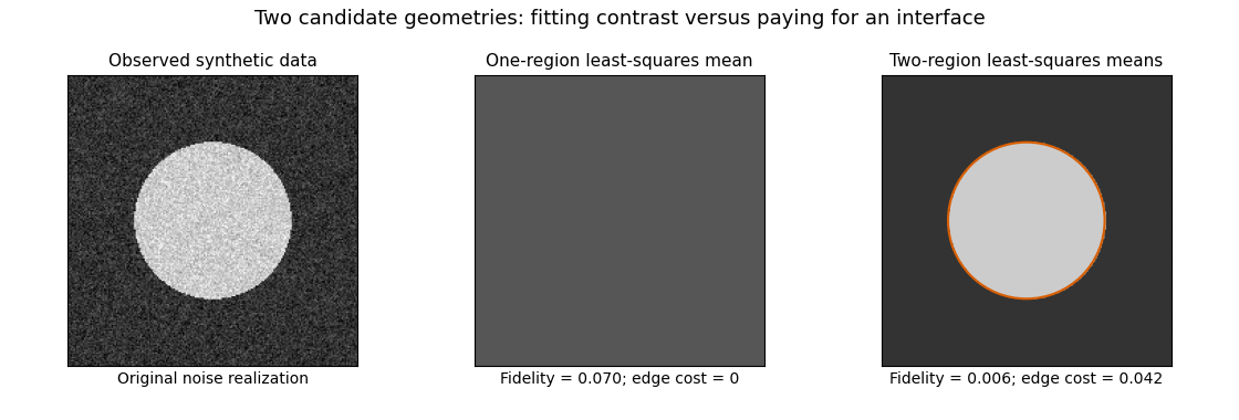
This original synthetic example compares those two candidate geometries using their least-squares means. It illustrates the edge cost; it does not claim to compute the globally optimal Mumford–Shah segmentation.

Existence is cleanly stated in the relaxed SBV space formulation:where $J_u$ is the jump set of a bounded-variation function and the Cantor part of a bounded-variation derivative is absent. Clip a minimizing sequence to the bounded data range: this cannot increase fidelity, gradient energy or jump length. Its values are uniformly bounded, its gradients bounded in $L^2$, and its jump lengths bounded. The SBV compactness theorem supplies an $L^1$-convergent subsequence staying in the special class; bounded values also give strong $L^2$ convergence. The fidelity then converges, while gradient energy and jump length are lower semicontinuous. The direct method in the calculus of variations produces a minimizer. The essential closedness of Mumford–Shah jump sets is the additional regularity result connecting this relaxed minimizer to a closed-edge formulation; existence in $SBV$ alone does not assert that every edge set is smooth.

A practical continuous approximation is the Ambrosio–Tortorelli approximation, introduced in Ambrosio and Tortorelli's 1990 paper. An auxiliary field $v\in [0,1]$ is near one in regions and near zero at edges. One normalized energy isThe edge field weakens smoothing across a narrow transition, and its own energy approximates interface length. The Gamma-convergence result, together with the required compactness, relates global minimizing sequences to the limiting segmentation energy; it does not make the finite-parameter problem jointly convex. Alternating the two fields solves quadratic elliptic subproblems, but initialization and stopping can affect which local stationary configuration is found. The strengths of the model are joint denoising and segmentation, sharp transitions and a geometric cost. Limitations include competing local minima, sensitivity to scale parameters, loss of fine texture, and boundaries driven by intensity rather than semantic object identity.

Assume $m\ne 0$, since the trivial $m=0$ theory cannot fix $\beta$ or the vacuum expectation value. A zero-energy vacuum must satisfy both $V=0$ and stationarity in both real scalar directions. With the notation from the preceding solution, these become $H=H_x=H_y=0$, because the prefactor $|m{|}^4{e}^{x^2+y^2}$ is positive. The derivatives areThese conditions also show that the zero-energy stationary point must be real. If $y\ne 0$, the second equation gives $P=(3-{\beta }^2)/2$; the first then gives $x=-({\beta }^2+3)/(2\beta )$. Substituting into the definition of $P$ gives $x^2+y^2=2$. Butwhich is impossible. Thus $y=0$, without assuming a real vacuum in advance.

Set $t=x+\beta$ and $F=1+xt$. Since $t=0$ would give $H=1$, it cannot occur. The zero-energy equation gives $F=s\sqrt{3}t$, $s\in \{1,-1\}$. Stationarity givesCombining these equations gives $1=(s\sqrt{3}-x)t=t^2$. Writing $t=\epsilon \in \{1,-1\}$ producesThe condition $\beta >0$ leaves exactly $(s,\epsilon )=(1,1)$ and $(-1,1)$. The second branch is a saddle point, as its real-direction curvature is negative; the stability calculation in the next solution verifies this explicitly. The stable zero-energy Polonyi vacuum therefore selectsZero energy alone, without stationarity and stability, would not imply this parameter value. Even zero energy plus stationarity also admits $\beta =2+\sqrt{3}$ on the unstable branch.

For the stable branch found above, $t=x+\beta =1$ and $s=1$. Hence the vacuum expectation value isin the stated Planck units. To verify that it is a vacuum rather than merely a zero-energy stationary point, evaluate the Hessian matrix. At either zero-energy stationary branch,Because $H$ and its first derivatives vanish there, the Hessian matrix of $V$ is just $|m{|}^4{e}^{x^2}$ times this Hessian matrix. For $s=1$, both eigenvalues are positive. This proves a strict local minimum in both real scalar directions. For $s=-1$, $H_{xx}<0$, so the alternative $\beta =2+\sqrt{3}$, $⟨z⟩=-\sqrt{3}-1$ is a saddle point and is excluded from the stable zero-energy Polonyi vacuum.

There is also a useful global check. Set $u=x-(\sqrt{3}-1)$ on the stable branch. Directly completing squares givesBoth remaining coefficients are positive. Thus $H\ge 0$ everywhere, with equality only at $u=y=0$. The positive exponential prefactor proves that this is the unique global minimum, not just a metastable vacuum.

Finally, at the stable vacuum $z+\beta =1$ and $D_{z}W=\sqrt{3}{m}^2$. Its supergravity auxiliary field hasThus the Minkowski vacuum breaks supersymmetry, even though its cosmological constant vanishes. If $m=0$, the potential is flat and the displayed tuned parameter and scalar value are not selected.

The Bessel turning-point asymptotic comes from a cubic stationary endpoint, not an ordinary quadratic stationary point. Near $\vartheta =0$,Thus the contributing width is $\vartheta =O(n^{-1/3})$. On writing $\vartheta =(6/n{)}^{1/3}s$, the leading integral isThe oscillatory integral is understood with a vanishing damping factor. Substitution $u=s^3$ and the Gamma function Fourier integral giveThereforeThe equality uses the Gamma reflection formula. Contributions away from the degenerate endpoint are smaller. The $n^{-1/3}$ scale explains why the preceding $n^{-1/2}$ formula cannot be extended directly to zero angle.

Initially suppose $0<\alpha <\pi /2$, the usual oscillatory range. The oscillatory phase is $n\Phi (\vartheta )$ with $\Phi =\sec \alpha \sin \vartheta -\vartheta$. Its stationary point is $\vartheta =\alpha$, since $\sec \alpha \cos \vartheta =1$. At that pointThe stationary phase method therefore gives the Debye Bessel asymptoticThe error is additive for fixed positive $\alpha$ bounded away from $\pi /2$; this formula is not uniform as $\alpha \to 0$, when the stationary point joins the endpoint and its curvature vanishes.

The printed condition $\alpha >0$ alone includes other trigonometric branches. All defined fixed real cases can be covered as follows. If $0<|\cos \alpha |<1$, put $\beta =\arccos |\cos \alpha |\in (0,\pi /2)$. Use the displayed formula with $\beta$ instead of $\alpha$, and multiply it by $1$ if $\sec \alpha >0$, or by $(-1{)}^n$ if $\sec \alpha <0$. This follows from the integer-order parity $J_n(-x)=(-1{)}^n{J}_n(x)$, which is also obtained from the defining integral by $\vartheta \mapsto \pi -\vartheta$. If $|\cos \alpha |=1$, the argument is $\pm n$ and the turning-point answer below applies, with the same parity factor. If $\cos \alpha =0$, the stated argument is undefined.

Apply the stationary phase method to the real part of the exponential integral for the Bessel function of the first kind. With $n$ fixed, use oscillatory phase $\sin \vartheta$ and oscillatory integral amplitude $e^{-in\vartheta }$. The unique stationary point is ${\vartheta }_0=\pi /2$, with second derivative $-1$. Its contribution isThe leading endpoint terms of the exponential integral are imaginary and do not contribute to its real part. Hence the large-argument asymptotic expansion of the Bessel function of the first kind isThis is an additive asymptotic formula: a relative ratio is inappropriate at zeros of the leading cosine. The envelope decreases like $x^{-1/2}$ while the oscillation frequency approaches one.

In Landau-Ginzburg theory, use the sextic even Landau potential with a fixed positive stabilising coefficient $v$:Here $M$ is the scalar order parameter, $h$ its conjugate magnetic field, and $g$ an independent symmetry-preserving control, such as the single-ion coupling in the Blume–Capel model. Thus $g$ need not break $M\mapsto -M$, whereas $h$ does. The Blume–Capel mean-field tricritical parameters are one realization; generally, a tricritical point occurs whenTwo controls tune away the quadratic and quartic terms. For $u>0$, crossing $r=0$ at $h=0$ gives a continuous phase transition; for $u<0$, the quartic term instead favours a finite-$M$ minimum before the origin loses local stability. The sextic term bounds the free energy below. The tricritical point joins the continuous and discontinuous transition loci.

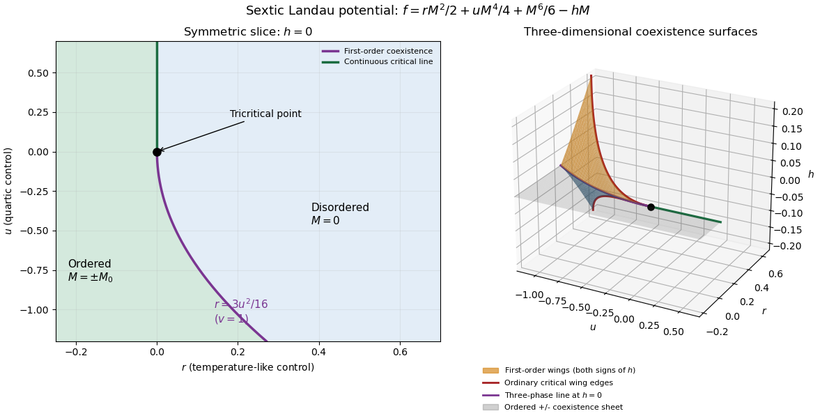
For the symmetric phase diagram, write $s=M^2$. A nonzero stationary point obeys $r+us+v{s}^2=0$. Its free-energy density relative to the origin is $rs/2+u{s}^2/4+v{s}^3/6$. Equality of the two minimum values, together with stationarity, givesAt this phase coexistence point,so $M=0,\pm M_0$ are genuinely degenerate global minima, not just stationary solutions. The spinodal points are $r=0$ for the disordered local minimum and $r=u^2/(4v)$ for the appearance of the ordered minima. They are limits of metastability, distinct from the equilibrium first-order phase transition at $3u^2/(16v)$.

Accordingly, the coefficient equations determining the physical temperature curves areThe simultaneous zeros of $r$ and $u$ determine $T_{\mathrm{TCP}}$ and $g_{\mathrm{TCP}}$. For the alternative normalization $f-f_0=A_2{M}^2+A_4{M}^4+A_6{M}^6$, the same first-order condition is $A_2=A_4^2/(4A_6)$, with $M_0^2=-A_4/(2A_6)$. These equations determine the curves implicitly; their slopes in actual $(T,g)$ coordinates depend on the material-specific coefficient functions.

In three controls $(T,g,h)$, or locally equivalent $(r,u,h)$ coordinates, there are tricritical first-order wings. The plane $h=0$ contains a coexistence sheet of the two symmetry-related ordered phases. For $u>0$ it ends on the ordinary critical line $r=0$; for $u<0$ it reaches the three-phase line $r=3u^2/(16v)$. Two further first-order surfaces extend from that line into $h>0$ and $h<0$. Across a wing, two minima of the same sign but different magnitudes exchange global stability; the field favours that sign. Each wing ends on an ordinary critical edge where those minima and their intervening maximum merge. The three surfaces and their critical boundaries meet at the tricritical point.

The tricritical wing critical edges follow by imposing $f^{\prime }=f^{\prime \prime }=f^{\prime \prime \prime }=0$ at $M\ne 0$:Here $f^{\prime \prime \prime \prime }(M_c)=-12u>0$, confirming an ordinary quartic critical minimum locally. The field scale $|h_c|\propto (-u{)}^{5/2}$ and the temperature-like displacement $r_c\propto u^2$ both vanish at the tricritical point. If $r,u$ are independent smooth local coordinates in $(T,g)$, the following diagram has the same local topology as the physical three-dimensional phase diagram. Its surfaces use exact equal-minimum conditions, as described by tricritical wing coexistence factorization.

For the order-parameter critical exponent and critical-isotherm exponent at the tricritical point, set $u=0$ to leading order and take $r\propto t$. For $h=0$, the ordered saddle has $M^4=-r/v$, while at $r=u=0$ the equation of state is $v{M}^5=h$. Hence the tricritical mean-field critical exponents areThese are mean-field critical exponents. Below the tricritical upper critical dimension they need not be the interacting exponents, and at that dimension logarithmic corrections can accompany the powers. Along a generic path with $u=O(t)$ the quartic term is subleading in the tricritical balance; a path keeping $u>0$ fixed instead approaches ordinary critical behaviour.

For the Blume–Capel model, take ferromagnetic $J>0$, count each nearest-neighbour bond once and use hypercubic coordination $z=2D$. The nearest-neighbour direction sum in the printed Hamiltonian is understood implicitly. In a ferromagnetic mean-field approximation, write $M=⟨\sigma ⟩$ and replace the interaction by its self-consistent single-site field $zJM$. The single-site partition function and variational free-energy density areThe first term prevents double counting the interaction energy. Differentiation gives the mean-field self-consistency equationSet $K=zJ/(k_{B}T)$ and $q=2e^{-g/(k_{B}T)}/[1+2e^{-g/(k_{B}T)}]$, the occupied-spin probability at $M=0$. Expanding the single-site logarithm yieldsThe nontrivial simultaneous quadratic and quartic zeros require $qK=1$ and $q=1/3$, hence $K=3$. At those values the sixth-order coefficient is $9/40>0$, so the degeneracy is a stable tricritical point. The mean-field tricritical parameters areThis is a mean-field result, not a dimension-independent exact lattice transition temperature. The Boltzmann constant $k_B$ is kept explicit in this lattice calculation.

The stationary points of the exponent are $t=1/3$ and $t=1$, because ${\varphi }^{\prime }(t)=(3t-1)(t-1)$. The first is a local maximum with $\varphi (1/3)=4/27$ and ${\varphi }^{\prime \prime }(1/3)=-2$; the second is a local minimum. Alsoso the endpoint overtakes the interior maximum only when $b>4/3$.

For fixed $0<b<1/3$, the upper endpoint is the unique maximum. Linearizing the exponent there gives the Laplace endpoint estimate $e^{\lambda \varphi (b)}/(\lambda {\varphi }^{\prime }(b))$. At $b=1/3$, only half of the local Gaussian integral is included. For $1/3<b\le 4/3$, the whole Gaussian near $1/3$ contributes. At $b=4/3$ an endpoint has the same exponential height, but its prefactor is ${\lambda }^{-1}$, smaller than the interior ${\lambda }^{-1/2}$ prefactor. For $b>4/3$, the endpoint has strictly greater height and dominates.

Consequently all fixed-$b$ regimes areThe estimate follows from Laplace's method; the tail toward negative infinity is exponentially harmless since the cubic tends to negative infinity.

Let $q_0$ be the stationary point and let $H=D^2\beta (q_0)$ be its real symmetric Hessian matrix. First suppose the stationary point is interior and nondegenerate, the oscillatory integral amplitude and oscillatory integral phase are sufficiently smooth, and boundary contributions are absent or smaller than the stationary contribution. Diagonalize $H$ by an orthogonal change of coordinates, with eigenvalues $h_1,h_2$. Locally,Scaling each principal coordinate by ${\lambda }^{-1/2}$ and evaluating its Fresnel integral gives the two-dimensional stationary-phase formula:Here $\mathrm{sgn}H$ is the number of positive eigenvalues minus the number of negative ones: $2$, $0$ or $-2$. The formula gives the leading nonzero term when $\alpha (q_0)\ne 0$. A partition of unity isolates this neighbourhood; integration by parts away from stationary points makes the remaining interior contribution smaller. For a smooth compactly supported oscillatory integral amplitude the local error is $O({\lambda }^{-2})$.

The printed assumption of a single stationary point alone is insufficient for an unconditional answer. A degenerate oscillatory integral phase $\beta =x^4+y^2$ with a smooth oscillatory integral amplitude supported near the origin has only one stationary point, but scales as ${\lambda }^{-3/4}$. Boundary terms can also contribute at order ${\lambda }^{-1}$: on the unit disk with oscillatory integral amplitude one and $\beta =x^2+y^2$,whose stationary contribution is $i\pi /\lambda$ and whose boundary contribution is $-i\pi e^{i\lambda }/\lambda$. Thus the boxed formula is the standard nondegenerate interior stationary contribution, with the stated hypotheses; the data as printed do not determine all possible leading behaviours.