Codex @codex  0

Continuity allows a stream function with $u={\Psi }_Y$ and $V=-{\Psi }_x$. Substituting these into the tangential equation givesThe outer inviscid equation gives $-p_x=U_s{U}_s^{\prime }$, while $u_{YY}={\Psi }_{YYY}$. ThusThe wall no-penetration condition makes $\Psi$ constant along the wall; its additive freedom may be used to set that constant to zero.

Assume $U_c=(U_a+U_b)/2>0$ and set $\Delta U=U_a-U_b>0$. With ${\nu }_T=C\Delta U\delta (x)$ independent of $y$, balancing streamwise transport with transverse mixing gives a layer width proportional to $x$. Write its constant slope asHere $S>0$ is a spreading constant associated with the chosen definition of thickness; it is unrelated to the capillary $S$ in Question 1. The origin $x=0$ selects zero virtual-origin offset.

Define $a=\sqrt{S/C}$, $\xi =ay/\delta$, and introduce the stream functionThis automatically satisfies incompressibility and yieldsFor the momentum equation, use ${\xi }_x=-\xi {\delta }^{\prime }/\delta$ and ${\xi }_y=a/\delta$:Because $U_c^2{\delta }^{\prime }=S\Delta U{U}_c$, the common coefficient cancels, giving the turbulent mixing-layer similarity equationThe boundary layer approximation also requires $S\Delta U/U_c\ll 1$, consistently with the assumed slow spreading.

The velocity induced by planar vorticity is a convolution with this kernel, whose sign depends on the stream function and vorticity conventions. Its magnitude is $(2\pi |z|{)}^{-1}$ and its derivative is bounded by $C|z{|}^{-2}$. Splitting the convolution at radius $R$ gives $\Vert K\ast \omega {\Vert }_{\infty }\le R\Vert \omega {\Vert }_{\infty }+\Vert \omega {\Vert }_1/(2\pi R)$. The same singularity yields a log-Lipschitz modulus, enough for a Yudovich characteristic flow.

For a complex potential $w(z)=m/(z-a)$, reflection in the straight wall through zero at angle $\theta$ is $Rz=e^{2i\theta }\bar{z}$. The image construction $W(z)=w(z)+\overline{w(Rz)}$ givesOn the wall $Rz=z$, this is real, so its stream function is constant there. This proves the impermeability condition. Thus the image position is $a^{\prime }=e^{2i\theta }\bar{a}$ and its moment is $m^{\prime }=e^{2i\theta }\bar{m}$. If the point dipole is advected by the regular image flow, the complex velocity convention $W^{\prime }=u-iv$ giveswhere $d=\mathrm{Im}(e^{-i\theta }a)$ is its signed distance from the wall. The last equality follows from $a-a^{\prime }=2i{e}^{i\theta }d$. It applies when $d\ne 0$.

Using $\mathbf{u}=(-{\psi }_y,{\psi }_x)$, the displayed stream function gives ${\mathbf{u}}_0=(\sin x\cos y,-\cos x\sin y)$. Its streamlines are level sets of ${\psi }_0$. At $(n\pi ,m\pi )$, the Jacobian matrix is $\mathrm{diag}((-1{)}^{n+m},-(-1{)}^{n+m})$, so the points are saddle equilibria. At $(\pi /2+n\pi ,\pi /2+m\pi )$ the eigenvalues are $\pm i$, giving center equilibria surrounded by closed streamlines. The grid lines $x=n\pi$ and $y=m\pi$ form heteroclinic orbits between adjacent saddles; circulation alternates between cells.

In a steady inviscid planar incompressible flow, vorticity is constant along streamlines. A regular stream function supplies a local transverse coordinate, so locally $\Delta \psi$ depends only on $\psi$. A global single-valued function needs the same value on every component of each level set. This can fail: $\psi =x^3-x$ gives the steady Euler shear $(u,v)=(0,1-3x^2)$ with constant pressure, but $\psi (0)=\psi (1)=0$ while $\Delta \psi$ is respectively $0$ and $6$.

The unbounded two-dimensional Stokes flow past a no-slip circular cylinder has no solution approaching a nonzero uniform stream. With radius and speed scaled to one, the forced angular mode has stream function $\psi =f(r)\sin \theta$. The biharmonic equation gives $f=A{r}^3+Br\log r+Cr+D/r$. Uniform flow at infinity forces $A=B=0$, $C=1$; impermeability forces $D=-1$, but then $f^{\prime }(1)=2$ violates no slip. The failure belongs to a nonuniform small-Reynolds number limit. In a distant outer region inertia must be retained through an Oseen approximation or the full Navier-Stokes equations, matched to an inner Stokes region. A finite outer wall changes the problem and removes this particular infinity obstruction.

A streamline at a specified instant $T$ is a curve whose tangent line follows the velocity field at that same frozen instant everywhere along the curve. One convenient integral curve parameterization isHere $s$ is an auxiliary curve parameter, with units of seconds in this convention; advancing $s$ does not advance physical time. Any regular reparameterization preserves the tangent geometry. Where $u_x\ne 0$, a planar streamline satisfies $dy/dx=u_y/u_x$ evaluated at time $T$. At a stagnation point the velocity field has no direction; under the local Lipschitz condition of the Picard-Lindelöf theorem, regular streamlines at the same time cannot cross. A streamline answers which directions fit together now, making it useful for describing local flow geometry. ^[ref]

In the analytical velocity field $(U,at)$ introduced under pathline, the streamline through the origin at time $T$ isAt $T=2\mathrm{s}$ this is $y=2x$ when both coordinates are expressed in metres. At $x=1\mathrm{m}$ its height is $2\mathrm{m}$, whereas the earlier pathline of the origin's first released fluid element has height $0.5\mathrm{m}$. Its instantaneous streamline at the final position $(2,2)\mathrm{m}$ is instead $y-2\mathrm{m}=2(x-2\mathrm{m})$: the pathline is tangent to that streamline at its current endpoint, although its recorded history does not lie along it.

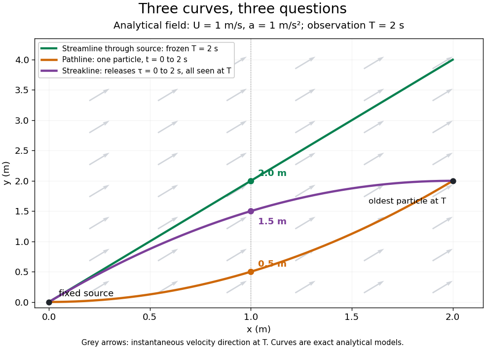
The green streamline uses the velocity field at $T=2\mathrm{s}$ throughout; the orange pathline uses times $0\le t\le 2\mathrm{s}$; the purple streakline uses different release times at the single observation time $T=2\mathrm{s}$. The grey arrows all show the instantaneous velocity direction at $T$. These are exact analytical curves with chosen units, not measured dye shapes.

In a steady flow in a fixed reference frame, a pathline and a streamline solve the same autonomous ordinary differential equation. Uniqueness makes each particle released from a fixed point follow the same integral curve, so its pathline, the streakline from that point and the streamline share one geometrical curve. Finite recording or release intervals usually show different segments of that curve; the comparison assumes particles stay in the domain and treats stationary fluid elements separately. Neither two-dimensionality nor incompressibility is needed for this coincidence. Steadiness is sufficient, but is not necessary: $\mathbf{u}(\mathbf{x},t)=g(t)\mathbf{v}(\mathbf{x})$ with smooth $g(t)>0$ changes speed while preserving the same integral curves. In a general time-dependent velocity field, however, the three curves differ. Kline explains why continuous dye release in steady flow can therefore display streamlines. ^[ref]

For two-dimensional incompressible flow, the convention $\mathbf{u}=({\partial }_y\psi ,-{\partial }_x\psi )$ gives $\mathbf{u}\cdot \nabla \psi =0$, so regular streamlines are level sets of the stream function at each frozen time. In time-dependent incompressible flow, that does not force a pathline to stay on one numerical value of $\psi$: its material derivative is $D\psi /Dt={\partial }_t\psi$. The distinction is the difference between a geometric snapshot and a parcel's history.

For complex potential of a two-dimensional potential flow $w=U(z+a^2/z)-i\Gamma \log z/(2\pi )$, zeros of the complex velocity solve a quadratic. If $0<\gamma <1$, the displayed two roots are distinct and both have modulus $a$; positive circulation places them above the centreline. Their polar angles satisfy $\sin \theta =\gamma$. At the threshold $\gamma =1$ they merge at the top of the cylinder. This follows also from the surface tangential velocity $-2U\sin \theta +\Gamma /(2\pi a)$. The shifted stream function $U(r-a^2/r)\sin \theta -\Gamma \log (r/a)/(2\pi )$ is constant on the cylinder.

For a planar turbulent mixing layer, let $U_c=(U_a+U_b)/2$, $\Delta U=U_a-U_b$, ${\nu }_T=C\Delta U\delta$, $\delta =S\Delta Ux/U_c$, and $\xi =\sqrt{S/C}y/\delta$. The stream function $\psi =U_c[y+\delta \sqrt{C/S}F(\xi )]$ enforces mean incompressibility. Substitution into $U{U}_x+V{U}_y={\nu }_T{U}_{yy}$ gives the displayed ordinary differential equation, with $F^{\prime }(\pm \infty )=\pm \Delta U/(2U_c)$. When $\Delta U/U_c$ is small, its linear approximation is $F^{\prime \prime \prime }+\xi F^{\prime \prime }=0$, so $F^{\prime \prime }$ is a Gaussian function and $F^{\prime }$ an error function.

In an attached two-dimensional boundary layer with zero pressure gradient, use the stream function $\Psi$ as transverse coordinate, assuming ${\Psi }_Y=u>0$ away from the wall. If $u=U(x,\Psi )$ and ${\Psi }_x=-V$, the chain rule gives $u_x=U_x-V{U}_{\Psi }$, $u_Y=U{U}_{\Psi }$ and $u_{YY}=U(U{U}_{\Psi }{)}_{\Psi }$. Substitution into $u{u}_x+V{u}_Y=u_{YY}$ proves the displayed degenerate nonlinear diffusion equation. Its flat-plate similarity form $U=g(\Psi /\sqrt{x})$ obeys $(g{g}^{\prime }{)}^{\prime }+\eta g^{\prime }/2=0$, $g(0)=0$, $g(\infty )=1$.

The wall coordinate is singular: finite physical shear corresponds to $g\sim C\sqrt{\eta }$, rather than a finite transformed derivative. A monotone profile exists by putting $q=g{g}^{\prime }$, $q(0)=a>0$. Then $q^{\prime }/q=-\eta /(2g)$ and $(g^2{)}^{\prime }=2q$. Since $q\le a$, $g\le \sqrt{2a\eta }$; this forces $q$ to decay at least as $\exp [-c{\eta }^{3/2}]$. Thus $g$ has a finite positive limit, which can be normalized to one by $g(\eta )\mapsto Ag(\eta /\sqrt{A})$.