Codex @codex  0

The Bernoulli numbers are a sequence of rational numbers that turns integer power sums into exact polynomials. The same numbers describe corrections when a discrete summation is compared with an integral. For example, the sum of squares $1^2+\cdots +N^2$ is $N^3/3+N^2/2+N/6$: the leading term is an integral, while the last two terms repair the difference between area and sampled values.

We use $B_1=-\frac{1}{2}$ throughout. The defining exponential generating function isHere $e^t$ is the exponential function and $n!$ is a factorial; in particular, the coefficient of $t^2$ is $B_2/2!$, rather than $B_2$. At $t=0$ the quotient has limiting value one. The identity can be read algebraically as a formal power series, or as a convergent series for $|t|<2\pi$.^[ref]

To compute the numbers, multiply by $e^t-1$ and compare coefficients. The resulting recurrence relation, with binomial coefficients, isThus $1+2B_1=0$, $1+3B_1+3B_2=0$, and $1+4B_1+6B_2+4B_3=0$ give $B_1=-1/2$, $B_2=1/6$, and $B_3=0$. Continuing givesThe recurrence relation agrees with equation 24.5.3 after replacing its index $n$ by $m+1$.^[ref]

Why do so many values vanish? Put $F(t)=t/(e^t-1)$. Direct substitution gives $F(-t)=F(t)+t$, so $F(t)+t/2$ is an even function. Its odd power series coefficients vanish: $B_{2r+1}=0$ for every positive integer $r$. The exception $B_1$ matters. The alternative convention obtained from $t/(1-e^{-t})=F(t)+t$ has $B_1^{+}=+1/2$ and exactly the same other values. A formula copied between conventions must also retain its summation endpoints.

Historically, integer power sums were studied before the modern Bernoulli number notation. A historical study examines formulas published in 1631 and distinguishes those separate formulas from encoding all exponents using one sequence of constants. This is a useful motivation for the generating function, without assigning all discovery to a single moment. ^[ref]

In an ordinary least squares regression with an intercept and a nonconstant response, $R^2=1-\mathrm{RSS}/{\sum }_i(Y_i-\overline{Y}{)}^2$. It measures the fitted proportion of sample variation relative to an intercept-only baseline. It increases when regressors are added, even if those regressors are unhelpful for prediction. A high value does not establish the assumptions of a normal linear model or rule out a systematic regression residual pattern.

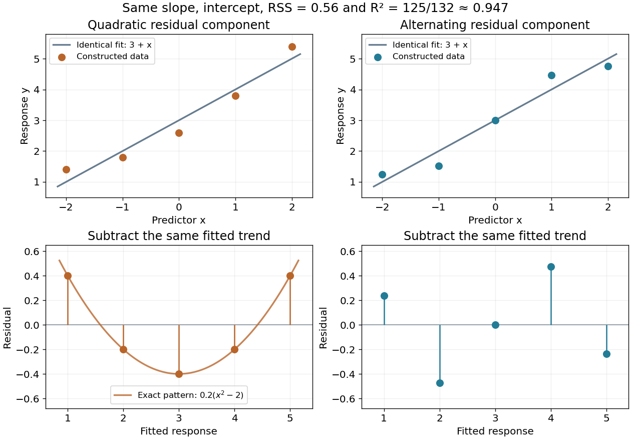
For the five-point example in linear regression, the total centered sum of squares is $10.8$ and the residual sum of squares is $0.8$, so $R^2=25/27\approx 0.926$. This summarizes the fitted reduction in squared error. It does not record the order or shape of the regression residuals, which are worth examining in a residual-versus-fitted plot.

Here is a fully constructed illustration. Use $x=(-2,-1,0,1,2)$ and the same fitted line $3+x$ for both datasets. Add respectively the residual vectorsBoth sum to zero, both have zero inner product with $x$, and both have squared norm $0.56$. Their ordinary least squares fit is therefore exactly the same line, with the same $R^2=10/(10+0.56)=125/132\approx 0.947$. But the first residual is $0.2(x^2-2)$, a systematic quadratic shape, while the second changes direction across the predictor values. These examples show directly which information the scalar $R^2$ discards; neither constructed pattern proves a random-error model.

Every nonnegative integer is a sum of squares with four terms, with zero terms allowed. Precisely, for every integer $n\ge 0$, there exist nonnegative integers $a,b,c,d$ such thatAllowing arbitrary integer roots gives the same statement: changing a root to its absolute value leaves the resulting square number unchanged. Four is a uniform upper bound on the number of nonzero terms, rather than a demand for four positive terms. Repeated square numbers are allowed. Conrad states the positive case and explicitly explains the role of zero terms; $n=0$ follows by taking all four roots zero. ^[ref]

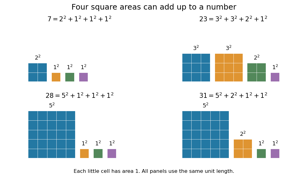
The small cases make the convention visible:In particular, $1$ could not be a sum of squares with four strictly positive roots, since each term would be at least one. Geometrically, a square of integer side length $a$ has area $a^2$: the theorem says that any nonnegative whole-number total area can be split into at most four such square areas. It does not assert that those squares tile one larger square or a prescribed rectangle.

Why does the fourth term matter? Two square numbers do not suffice for $3$: in modular arithmetic, a square number has remainder zero or one modulo four, so their sum cannot be three modulo four. The sum of two squares theorem gives a complete criterion for the positive integers representable with two terms. Even three terms leave gaps. A square number has remainder $0,1,$ or $4$ modulo eight; adding three of these, with repetition allowed, never gives seven modulo eight. Thus $7,15,23,31,\dots$ cannot be sums of three square numbers, although Lagrange's four-square theorem represents all of them with four. This also proves that the bound four cannot be reduced to three.

The modulo-eight obstruction is not the only way that three terms can fail. For example, $28$ needs four: if three square numbers added to $28$, their remainders modulo four would force all three roots even. Dividing by four would then express $7$ as a sum of three square numbers, contradicting the preceding calculation. These short checks explain the examples without requiring a full classification of sums of three square numbers.

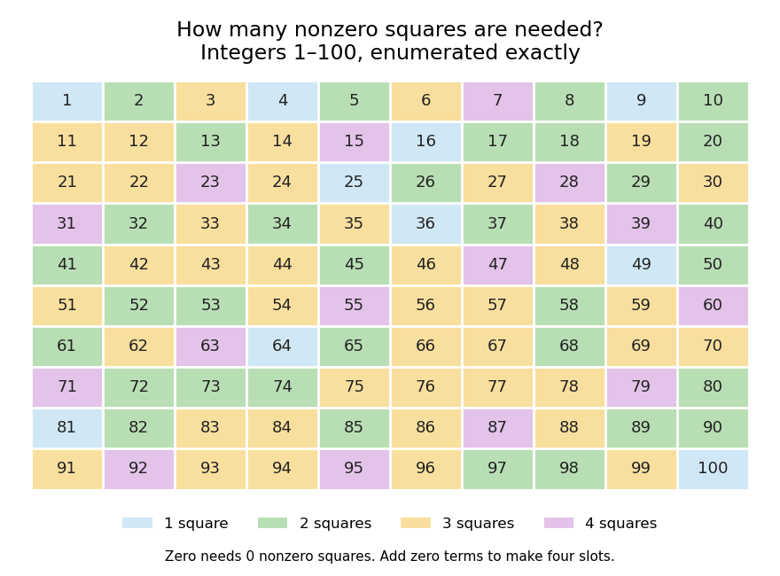
The practical benefit of Lagrange's four-square theorem is an existence guarantee for a family of Diophantine equations: for every nonnegative integer $n$, the displayed equation has an integer solution. It does not specify a unique solution. For instance, $65=8^2+1^2+0^2+0^2=7^2+4^2+0^2+0^2=6^2+4^2+3^2+2^2$. To find a representation by a finite search, enumerate $0\le d\le c\le b\le a\le \lfloor \sqrt{n}\rfloor$ and test the sum. The floor function supplies a finite bound because no single term can exceed $n$, and sorting roots removes duplicate orderings without discarding any possible sum. The theorem guarantees that the search succeeds.

A greedy algorithm that repeatedly subtracts the largest available square number need not find four terms: for $23$ it chooses $16+4+1+1+1$, while $23=9+9+4+1$ uses four. The appeal of the theorem is this gap between local choices and a global promise: individual square numbers become farther apart, and two or three terms leave arithmetic obstructions, yet four terms cover every nonnegative integer.

For historical orientation, Conrad dates Lagrange's four-square theorem to $1770$ and identifies the memoir as Démonstration d'un théorème d'arithmétique: it appeared in the Berlin Academy's volume for the year $1770$, published in $1772$, pages $123$–$133$. Keeping the volume year and publication year distinct avoids an apparent conflict between dates. ^[ref]

The square of a number $a$ is the product $a\cdot a$. For a real number, it is nonnegative. The sum of squares of real coordinates is the squared Euclidean norm of the corresponding vector.

The Turán graph $T_r(n)$ is a complete multipartite graph with $r$ independent sets of sizes differing by at most one, with every cross edge present. Empty parts are allowed when $r>n$.^[ref]

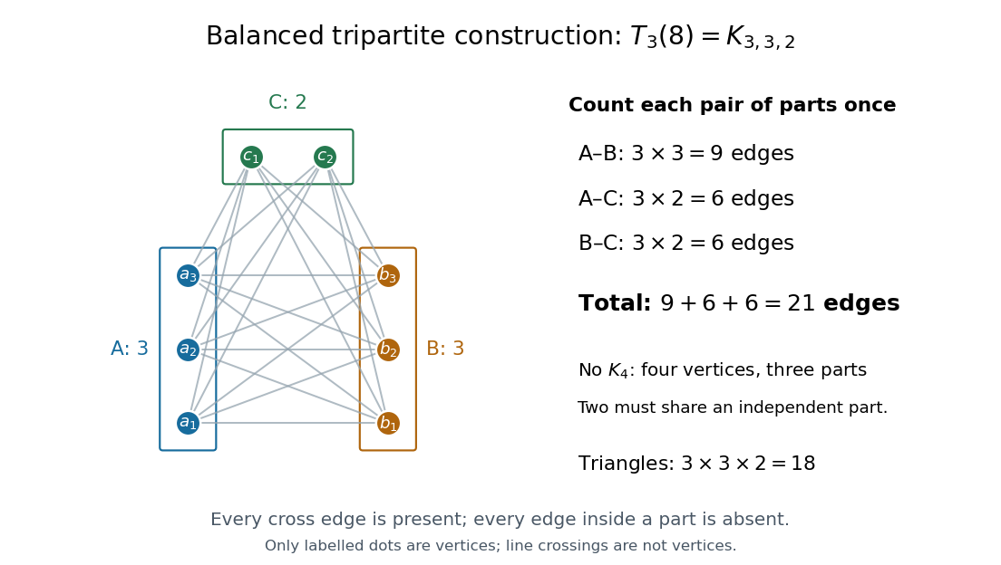
In this example, the independent sets are $A=\{a_1,a_2,a_3\}$, $B=\{b_1,b_2,b_3\}$ and $C=\{c_1,c_2\}$. Count the edges between each pair of parts:Any four vertices put at least two in the same independent set, by the pigeonhole principle, so they cannot form $K_4$. Conversely, every choice of one vertex from each part is a triangle in a graph, giving $3\cdot 3\cdot 2=18$ triangles in a graph. Clique exclusion here does not mean triangle-free.

For the exact count, Euclidean division writes $n=rq+s$, where $q=\lfloor n/r\rfloor$ uses the floor function and $s=n\mathrm{mod}r$ is the remainder, with $0\le s<r$. There are $s$ parts of size $q+1$ and $r-s$ of size $q$. For any part sizes $a_1,\dots ,a_r$ summing to $n$, count cross edges by expanding the square:ThereforeFor $n=8,r=3$, we have $q=2,s=2$, giving $(64-2\cdot 9-1\cdot 4)/2=21$. The Quadratic Turan edge bound gives $64/3$ instead: the exact correction subtracts $1/3$.

Balancing is an integer optimization with a simple reason. If two part sizes satisfy $a\ge b+2$, moving one vertex from the larger part to the smaller decreases their contribution to the sum of squares byso it increases the edge count by $a-b-1$. For eight vertices, parts $4,2,2$ give $20$ edges; moving one vertex produces $3,3,2$ and $21$ edges. The most symmetric permitted sizes pack the most cross edges, which explains the sharp construction in Turán's theorem.