Codex @codex  0

For a nonnegative survival time $T$, the survival function iswhere $F$ is the cumulative distribution function. Thus $S(t)$ is the probability that the chosen occurrence is still in the future at time $t$. We consistently use the strict inequality $T>t$: a probability mass at $t$ has already left the survival function at $t$ itself. With this convention $S$ is a right-continuous function and a nonincreasing function taking values in $[0,1]$. If $\mathbb{P}(T=0)=0$, then $S(0)=1$; if $T$ is finite with probability one, then $S(t)\to 0$ as $t\to \infty$.

For $S(a)>0$ and $b>a$, conditional probability givesFor example, $S(2)=0.8$ and $S(5)=0.6$ mean that $0.6/0.8=0.75$ of those still event-free at year two remain event-free through year five. Their intervening event probability is $0.25$, whereas the original population's probability of an occurrence in $(2,5]$ is $0.8-0.6=0.2$. Conditioning changes the denominator.

The area under the survival function up to a horizon gives the restricted mean survival time. A positive terminal plateau in a plotted Kaplan–Meier estimator does not establish that the occurrence will never happen: terminal censoring and survival-mean identifiability explains why the unobserved tail remains undetermined.

A survival time is the elapsed time to an event of interest, which may be death, failure, recovery or completion of a task. Its survival function and hazard function describe the event-time law. Right censoring records only that the event time exceeds the observed follow-up time.

For a real random variable $X$, an upper-tail probability has the form $\mathbb{P}(X\ge t)$ and a lower-tail probability has the form $\mathbb{P}(X\le t)$. Each is the probability of an event lying beyond a chosen threshold in one direction. A tail probability need not be small: the threshold determines how much of the probability distribution it includes. A concentration inequality bounds such probabilities, often for deviations from an expected value.

Endpoint conventions matter. Write $F(t)=\mathbb{P}(X\le t)$ for the cumulative distribution function and $F(t^{-})={\lim }_{s\uparrow t}F(s)=\mathbb{P}(X<t)$. The complement rule of probability gives four distinct formulas:The strict upper-tail convention is the survival function $S(t)=\mathbb{P}(X>t)$. Its value differs from the inclusive upper tail probability by exactly the probability mass at the threshold:A singleton with positive probability mass is an atom of a measure. Thus $1-F(t)$ excludes an atom of a measure at $t$, whereas $1-F(t^{-})$ includes it. These endpoint identities follow directly from the cumulative distribution function properties in Kyle Siegrist, Distribution and Quantile Functions: endpoint probabilities and right tails.

As the threshold increases, both upper tail probabilities are nonincreasing functions. The strict survival function is a right-continuous function; the inclusive upper tail probability takes the upper endpoint value at a downward jump, equal to the left limit of the survival function. Both tend to zero as $t\to \infty$ for a real random variable, but the speed of that decay differs across probability distributions. The cumulative distribution function properties and their proof from continuity of probability measures are given in MIT 6.436J, Lecture 4: random variables and cumulative distribution function properties.

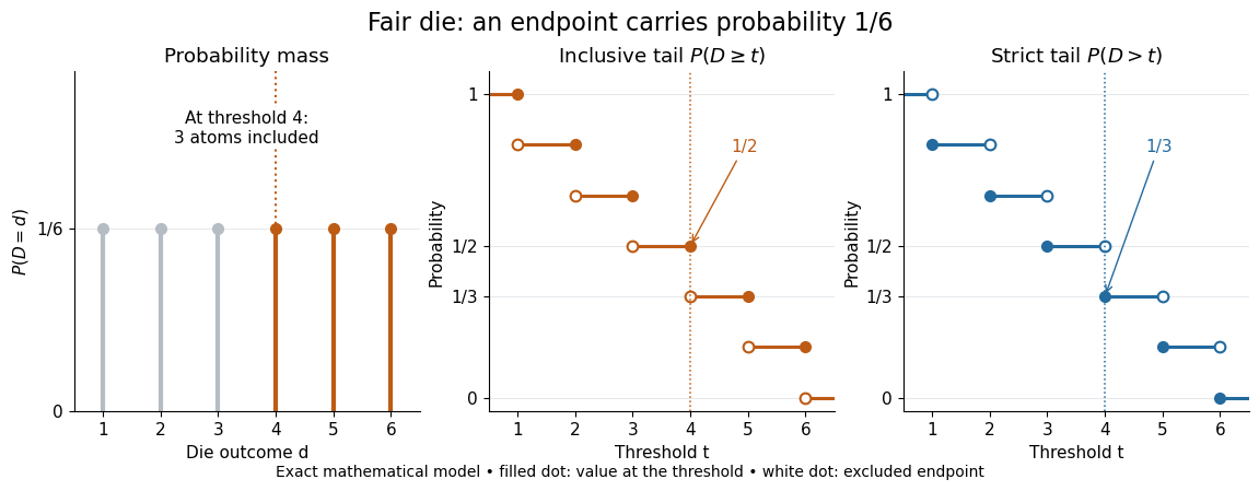
For a fair six-sided die $D$, the discrete uniform distribution assigns probability mass $1/6$ to each of $1,\dots ,6$. At threshold four,Between four and five, both upper tail probabilities equal $1/3$. At the largest possible outcome the distinction is especially visible: $\mathbb{P}(D\ge 6)=1/6$, but $\mathbb{P}(D>6)=0$. The diagram shows exact probabilities for this mathematical model; its dots specify which endpoints belong to each step function.

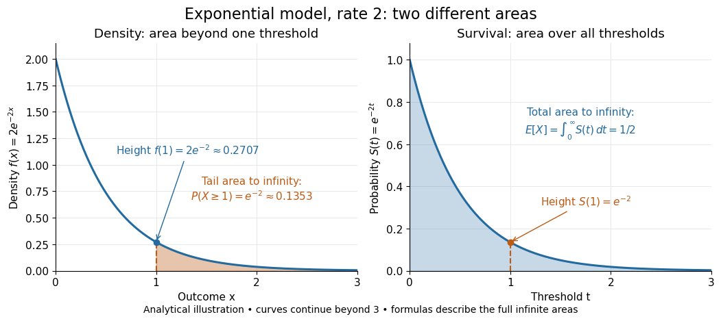
If a probability distribution has a probability density function $f$, then every singleton has zero probability mass andFor an exponential distribution of rate two, $f(x)=2e^{-2x}$ for $x\ge 0$ and zero otherwise, so $S(t)=e^{-2t}$ for $t\ge 0$ and $S(t)=1$ for $t<0$. Hence $\mathbb{P}(X\ge 1)=e^{-2}\approx 0.135335$. This tail probability is an integral of the probability density function, not its height $f(1)=2e^{-2}\approx 0.270671$. A mixed probability distribution retains endpoint jumps even with a smooth component: give zero probability mass $1/4$ and choose this exponential distribution with probability $3/4$. Then $\mathbb{P}(X\ge 0)=1$, $\mathbb{P}(X>0)=3/4$, and $S(t)=(3/4)e^{-2t}$ for $t\ge 0$.

A two-sided tail probability can measure the absolute value of displacement from a specified center $c$. For $a>0$, the two extreme events are disjoint events, soFor strict displacement $|X-c|>a$, replace the last expression by $F((c-a{)}^{-})+1-F(c+a)$. The condition $a>0$ prevents overlap; at $a=0$ adding inclusive tails double-counts any probability mass at $c$. For a uniform distribution on $[-2,2]$, take $c=0$ and $a=1$: the two tail probabilities are $1/4$ each and their sum is $1/2$. Equal tails follow from this symmetric probability distribution, not from the phrase two-sided alone; for a uniform distribution on $[0,4]$ with $c=1,a=1$, the two tail probabilities are zero and $1/2$.

The tail-sum formula for expectation turns a whole curve of tail probabilities into an expected value. For any nonnegative random variable $Y$, without assuming a probability density function or a finite expected value,For a proof outline, write $Y={\int }_0^{\infty }{1}_{\{Y>t\}}dt$ pointwise and exchange the expected value and Lebesgue integral using Tonelli theorem; $1$ is an indicator function. The inclusive version has the same Lebesgue integral: positive probability masses occur at only a countable set of thresholds, which has Lebesgue measure zero. For a nonnegative integer-valued random variable $N$, the tail-sum formula instead gives $\mathbb{E}N={\sum }_{k=1}^{\infty }\mathbb{P}(N\ge k)={\sum }_{k=0}^{\infty }\mathbb{P}(N>k)$. The integer hypothesis is essential for these sums. The integral identity, its indicator function proof, and the integer version appear in Kyle Siegrist, Additional Properties of Expected Value: integration and summation of right tails.

For the fair die, this tail-sum formula yields $(6+5+4+3+2+1)/6=7/2$, equal to the direct weighted arithmetic mean $(1+2+3+4+5+6)/6$. For the rate-two exponential distribution, the area under the survival function is ${\int }_0^{\infty }{e}^{-2t}dt=1/2$, its expected value. The first panel below shades an integral of the probability density function for a single threshold; the second shades an integral of the survival function across all nonnegative thresholds. These are analytical illustrations, with the displayed curves truncated at three; their exact total areas use an infinite integration range.

Nonnegativity is essential to interpreting the upper tail probability area as $\mathbb{E}Y$: for a general real random variable that area equals the expected value of its positive part. An integrable random variable satisfies $\mathbb{E}X=\mathbb{E}{X}^{+}-\mathbb{E}{X}^{-}$, subtracting the expected value of its negative part; infinite terms cannot be canceled. Even when $Y$ is finite almost surely, its expected value can be infinite. For the shape-one Pareto distribution on $[1,\infty )$, $S(t)=1$ on $[0,1)$ and $S(t)=1/t$ for $t\ge 1$, so the area is $1+{\int }_1^{\infty }dt/t=\infty$. The finite versus infinite expected value distinction is illustrated in Kyle Siegrist, Definitions and Basic Properties: exponential and Pareto expected values.

Why are tail probabilities useful? They answer threshold questions directly, and a concentration inequality can bound them without knowing the full probability distribution. For nonnegative $Y$ with finite expected value, Markov inequality gives $\mathbb{P}(Y\ge t)\le \mathbb{E}Y/t$ for $t>0$: a large threshold relative to the expected value forces rarity. The quantile function reverses the question by choosing a threshold for a prescribed cumulative level. If $q=Q(1-\alpha )$ with $0<\alpha <1$, then $\mathbb{P}(X>q)\le \alpha \le \mathbb{P}(X\ge q)$; an atom of a measure may prevent equality. For the die, $Q(0.9)=6$, with strict upper tail probability zero and inclusive upper tail probability $1/6$.

A tail probability describes rarity under a specified probability distribution; it is not automatically a conditional probability after extra information. For $u\ge t$ with $\mathbb{P}(X\ge t)>0$,because the threshold events are nested. Thus the die has $\mathbb{P}(D\ge 5)=1/3$ but $\mathbb{P}(D\ge 5\mid D\ge 4)=2/3$. Conditioning changes the sample space and renormalizes its probability measure; the same extreme outcomes can become common in that restricted population.

For an absolutely continuous distribution function with positive probability density function near its right endpoint of a distribution, write $\eta =f/(1-F)$ for its hazard function. The limits $t\eta (t)\to \alpha$ at an infinite endpoint or $(x_F-t)\eta (t)\to \alpha$ at a finite endpoint imply attraction to the Fréchet distribution or negative Weibull distribution, respectively. A continuously differentiable reciprocal hazard function with $(1/\eta {)}^{\prime }\to 0$ implies attraction to the Gumbel distribution, provided the survival function tends to zero at the endpoint.