A concentration inequality bounds the probability that a random variable differs substantially from a typical value such as its expected value or median.
Equip the symmetric group with its uniform probability measure and unnormalized Hamming distance. If has Lipschitz constant , it obeys the displayed two-sided bound, and each one-sided tail has the same exponential without the factor two. Reveal a uniform permutation one image at a time. Two possible next images have completion sets paired by swapping those two values, changing exactly two coordinates. Thus the corresponding conditional means differ by at most . Each increment of the Doob exposure martingale has conditional range length at most . Applying the conditional Hoeffding lemma gives ; optimizing the exponential Markov bound proves the bound. A mere absolute-increment bound of gives a weaker constant, so using the range length matters.
For an event in a product of finitely many probability spaces with its product measure, take the closed convex hull of the mismatch vectors , . The distance of this hull from zero is . Equivalently it is the supremum, over nonnegative coordinate weights of squared sum at most one, of their minimum mismatch sum. Averaging mismatch patterns is the feature that distinguishes this quantity from ordinary Hamming distance.
On a finite product of standard probability spaces, for any measurable event of positive probability,Consequently . Here is the Talagrand convex distance. The distance-event conclusion can be read with outer probability when necessary.
Let the largest last-coordinate section have probability , and another section probability . Mix mismatch vectors from these two sections with weights . Their squared norm is at most . Hölder's inequality and induction bound that section's exponential integral by . The scalar estimate for Talagrand product induction makes it at most . Average over sections and use with to close the induction.
For ,where the endpoint is used directly if . Put . For , choose and set . Then and , proving the bound. For , take ; the result follows from the already proved boundary case and monotonicity of . This estimate closes the section-by-section induction for the exponential Talagrand convex distance moment.
For a nonnegative integrable random variable , the entropy functional isIt is the unnormalized relative entropy of the measure with density proportional to relative to the original probability measure.
Here for a probability measure. The coefficient depends on the normalization of the energy. With the joint energy for , standard Gaussian measure has optimal constant two.
// Target: analysis.bigb
Differentiate with and a changing exponent. The derivative is . Apply the logarithmic Sobolev inequality to and the power inequality for symmetric Markov energies. Choosing makes the upper bound zero.
// Target: probability-and-statistics.bigb
The Hoeffding inequality turns finite interval bounds and independence into exponentially small tail probabilities for a sum. It requires neither a normal distribution nor identical probability distributions. Let be independent essentially bounded real random variables, with deterministic finite bounds almost surely. Define the centered sum and its squared-width budget byFor and ,The union bound therefore gives . If , every is constant almost surely, so and both positive-threshold tail probabilities vanish. The equal-width version is stated in the authored Stanford notes.[ref]
The quantity is a sum of squared interval widths, not the variance of . Centering changes the endpoints to and , leaving each width unchanged. For example, independent random variables in and have , whatever their expected values or probability distributions. A deviation at least three above their total expected value has probability at most . If all widths equal , the sample mean satisfies
Independence is essential to this general guarantee. Take one Bernoulli random variable with success probability and set every . Each lies in , but for every the sample mean is either zero or one. Thus , whereas incorrectly inserting these dependent observations into the formula would give , less than one for . Some special dependent models have their own valid concentration inequalities; arbitrary statistical dependence cannot be ignored.
For the short proof, apply Markov's inequality to with , factor the expectation using independence, and apply the Hoeffding lemma to each factor:Minimizing this quadratic polynomial at gives the upper tail probability; applying it to gives the lower one. This is the Chernoff bound method. The original 1963 article is Probability Inequalities for Sums of Bounded Random Variables by Wassily Hoeffding; its publisher record identifies the article, but its full text was unavailable during this source check. The argument above is a direct derivation rather than a claim to have inspected that article's proof.
Let be independent and identically distributed Bernoulli random variables with success probability , and let be their observed frequency, a sample mean. Since every interval width is one, . Substituting into the Hoeffding inequality givesFor tolerance and failure probability , solving yields the sufficient sample sizeHere is the natural logarithm. For and , guarantees an error smaller than with probability at least , for every . The two-sided bound at this sample size is approximately . A specified single direction instead needs , or for these choices. Halving the tolerance multiplies the unrounded sufficient sample size by four; reducing the failure probability tenfold adds before rounding.
This is a conservative sufficient sample size, not a necessary minimum. For a specified , the count has a binomial distribution, whose exact upper tail probability isFor , the Hoeffding inequality bounds this by . An arbitrary frequency threshold uses ; if , the event is impossible. The discreteness of the count and its variance can make the exact tail probability substantially smaller. At , , , the exact upper tail probability is about , while the bound is . At , , the same deviation gives the same bound but an exact upper tail probability about .
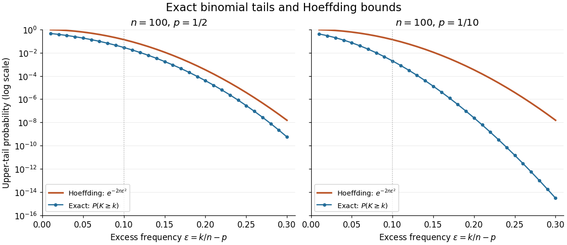
Exact binomial distribution tails compared with the Hoeffding inequality
. Two original specified models, each with independent Bernoulli trials. Each dot includes its integer threshold , with horizontal coordinate . Exact finite sums are evaluated with rational arithmetic before conversion for plotting. The Hoeffding inequality uses the width one in both panels; it does not use the smaller variance at . These are model probabilities, not measured frequencies. Details.For a fixed positive sample size of independent and identically distributed Bernoulli random variables, letThe Hoeffding inequality makes a conservative confidence interval for : for every . Indeed, exclusion from the closed interval implies , an event contained in the deviation event bounded by . Clipping to retains coverage because already lies there. For , , and an observed frequency , , giving approximately .
Coverage concerns repeated independent samples: the unknown is fixed and the confidence interval is random. This fixed- guarantee does not justify repeatedly checking the same bound and stopping as soon as it looks favorable. The Hoeffding sample size for Bernoulli frequencies chooses in advance; guarantees across repeated inspection times require separate control of the additional events, for example through a union bound with an allocated failure probability at each time.
The Hoeffding lemma controls the entire centered moment-generating function using only an interval width. For an essentially bounded real random variable with finite deterministic bounds almost surely, every real satisfiesEquivalently, . This single-random variable statement needs no independence assumption; independence enters when applying it to the factors for a sum in the Hoeffding inequality. Both signs of are allowed, and equality holds at or when .[ref]
In the convention for a centered sub-Gaussian random variable , the Hoeffding lemma supplies . This upper parameter need not equal the actual variance. For a Bernoulli random variable of success probability ,The actual variance is , whereas the supplied parameter is for every . This explains part of the conservatism visible in Hoeffding sample size for Bernoulli frequencies.
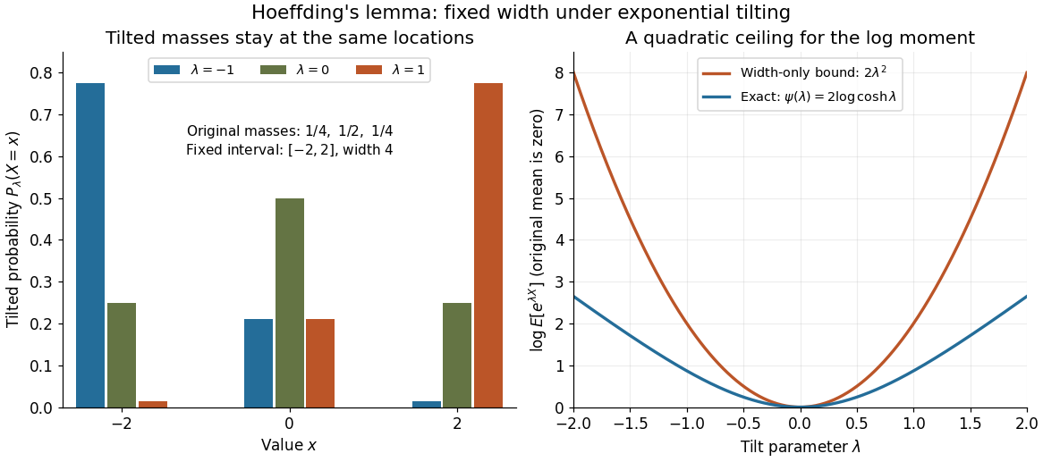
A short proof exposes why the constant is . Put and define exponential tilting byThe tilted probability measure has the same interval of possible values, and differentiating the cumulant-generating function gives . Boundedness justifies these derivatives for every finite . Under any such tilted law, Popoviciu's inequality on variances gives : the variance is no larger than the expected value of the squared distance from the interval midpoint, itself at most . Since , the integral form of Taylor's theorem yieldsThis expression handles either sign of without changing the argument.
The constant cannot be reduced uniformly over all essentially bounded real random variables. Equal endpoint probabilities at and give , a scaled Rademacher random variable, andThus the sharpness is already forced near zero by the variance; the bound need not be equality at nonzero parameters for a particular probability distribution.
For a binomial distribution with and , the Bennett inequality at standard deviations tends to , whereas the Hoeffding inequality tends to two. The raw Bennett inequality bound is eventually smaller for any fixed ; after clipping at one it is nontrivial in the limit only when .
The Bennett rate function has Taylor expansion near zero. It is the optimized exponent in the Chernoff bound based on the moment-generating function estimate for the Bennett inequality.
If each probability measure has Poincaré constant , then the product measure has Poincaré constant at most . This follows by iterating the law of total variance and applying Jensen inequality to derivatives of conditional expectations.
If has Poincaré constant and is -Lipschitz, then the pushforward measure has Poincaré constant at most . Apply the original inequality to and use the chain rule.
For the uniform distribution on ,The constant is sharp and is the mean-zero Poincare-Wirtinger inequality on the interval.
For standard one-dimensional Gaussian measure, . Thus , while . Every nonzero therefore attains ratio two, proving optimality of the Gaussian constant.
For bounded smooth positive bounded away from zero, differentiation and Gaussian integration by parts give the displayed identity. The Ornstein-Uhlenbeck gradient commutation identity and weighted Cauchy-Schwarz inequality bound its right side by . Integrating and setting proves the Gaussian logarithmic Sobolev inequality. Positive clipped approximation extends it to functions of finite Gaussian Dirichlet energy.
For every , Markov inequality applied to givesOptimizing over gives the Chernoff bound in terms of the moment-generating function of .
For a matrix of independent standard normal entries and , diagonal entries of have two-sided tails bounded by , while off-diagonal entries have tails bounded by . A union bound over diagonal entries and distinct off-diagonal entries controls their common entrywise maximum norm.
If are independent random variables and has bounded differences constants , thenand the same bound holds for the lower tail.
For a nonempty of relative size at least , its Hamming distance function has the bounded differences property with all constants one. If , the concentration bound at gives , so for . Then , proving that the radius- neighbourhood contains at least cube points.
If a function of independent coordinates has one-sided squared-difference proxy at most , Talagrand's one-sided inequality gives a Gaussian lower-tail bound . Applied to the negative of a concave function, it gives the corresponding upper-tail bound.
An integer-valued function is -certifiable when every input with has a set of at most coordinates whose values alone guarantee that .
The entropy method combines a coordinatewise certificate with tensorization of entropy to bound the moment-generating function of a certifiable random quantity and hence its tails.
A nonnegative function of independent coordinates is self-bounding when there are coordinate-deleted versions such that andThese inequalities make the natural variance proxy no larger than the function itself.
A nonnegative function is weakly self-bounding when coordinate-deleted functions satisfy andThe squared coordinate sensitivity is then controlled by the observed value of the function itself.
For a weakly self-bounding function of independent random variables, the coordinatewise variance inequality giveswhere .
For a nonnegative function of independent random variables, entropy is at most the sum of its conditional coordinate entropies. This tensorization is a basic step of the entropy method.
For independent coordinates and square-integrable ,For Bernoulli coordinates, each conditional variance is an explicit squared coordinate difference.
A modified logarithmic Sobolev inequality bounds the entropy of by a one-sided coordinate-difference energy. For independent coordinates and arbitrary coordinate-deleted functions , tensorization givesIf that energy is at most , one common normalization is
The Herbst argument integrates a logarithmic Sobolev bound on to control the centered cumulant-generating function , then applies a Chernoff bound to obtain concentration.
A transport-entropy inequality controls an optimal expected transportation cost between probability distributions by their Kullback-Leibler divergence.
If each coordinate law satisfies the same convex transport-entropy inequality, then the product law satisfies the sum-cost version. Sequentially couple conditional coordinates, apply Jensen inequality, and use the chain rule for relative entropy.
A centered random variable is sub-Gamma in the right tail with variance parameter and scale parameter whenfor .
Suppose independent centered sub-exponential random variables satisfy for , and put . Independence adds the log moment-generating functions. The Chernoff bound with gives the displayed two-sided tail. If each variable has common scale , one may take and , giving . This form of Bernstein's inequality allows unbounded variables with factorial moment control, including the centered square of a sub-Gaussian random variable.
For independent centered variables and , the th moment of their sum is bounded, up to a constant depending only on , by the sum of their th moments plus the power of their total variance.
Talagrand's concentration inequality gives strong concentration in product spaces using convex distance. If has positive product probability, its convex-distance enlargement has Gaussian tails. A Talagrand concentration inequality for certifiable functions follows by bounding this distance using bounded differences and small certificates.
This is an application of Talagrand's concentration inequality to certifiable functions. Talagrand's product-space inequality gives sub-Gaussian-type concentration for a bounded-differences, certifiable function, with a variance scale controlled by the certificate size.
Suppose an integer-valued certifiable function is -Lipschitz under one-coordinate changes and a value at least has a certificate of at most coordinates. Any input with value at most must differ on at least certificate positions. Equal weights on those positions bound its Talagrand convex distance from the low-value event. Applying Talagrand's convex distance inequality gives the displayed product bound. For , median tails integrate to , and deviations of order have exponentially small probability.
For the longest increasing subsequence length on a product space of independent coordinates, a witness of length uses only coordinates. Any point with subsequence length at most must differ on at least witness positions. Weights on those positions show . Thus for ,At a median , this gives upper tail and lower tail . Integrating the tails places the mean within of the median, so the natural concentration scale near the mean is . A random permutation is represented by the ranks of independent continuous variables; arbitrary dependent sequences need not obey this conclusion.
Articles by others on the same topic



Concentration inequalities are mathematical inequalities that provide bounds on how a random variable deviates from a certain value (typically its mean). These inequalities are essential in probability theory and statistics, particularly in the fields of machine learning, information theory, and statistical learning, because they help analyze the behavior of sums of random variables, as well as the performance of estimators and algorithms. There are several well-known concentration inequalities, each suitable for different types of random variables and different settings.